1 Introduction
Here we explore the viability of modelling the price of Chicago and Kansas City Wheat as a function of stock-to-usage. The market receives new information about the state of global stocks once a month after the WASDE reports have been published. As the global balance sheets change during the course of the season the expectation of the stock levels left over at the end of the season changes. We aim to model the Chicago and Kansas City Wheat prices along the futures curve as a function of stock-to-usage percentages of the major producing and consuming nations. We add a proxy for energy by looking at the average WTI crude price during the prior month. Furthermore we also consider the dollar strength as measure by the dollar index.
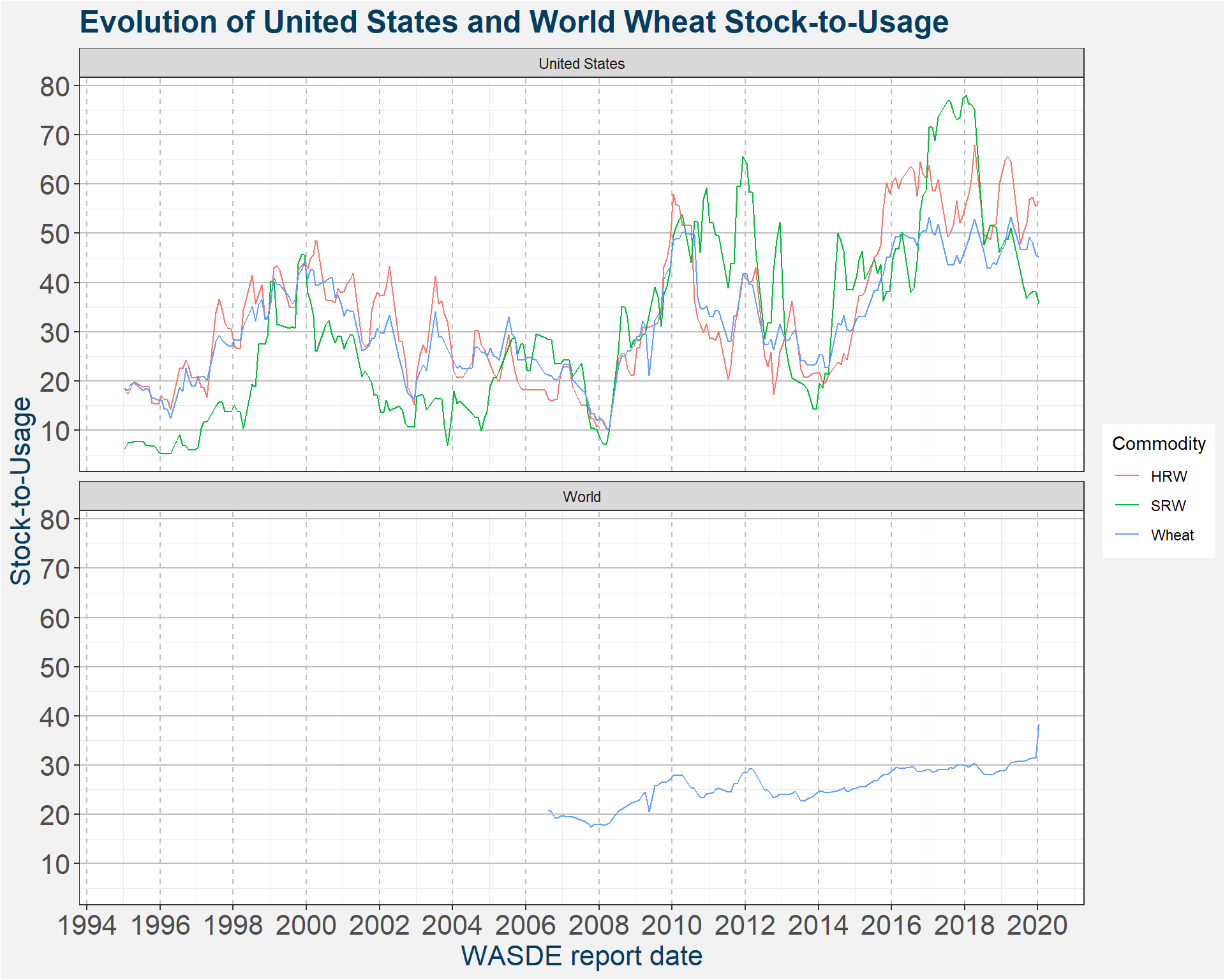
The plot below shows the evolution of the wheat stock-to-usage numbers for the United States and World levels. The different colours represent different classes of wheat.
We want to connect these stock-to-usage numbers with price of the corresponding wheat futures contracts. To do this we connect the price data between two successive WASDE reports with the first report and aggregate the results. As an example consider two reports dated 2018-05-11 and 2018-06-12 respectively. All price data between those two dates are associated with the first date.
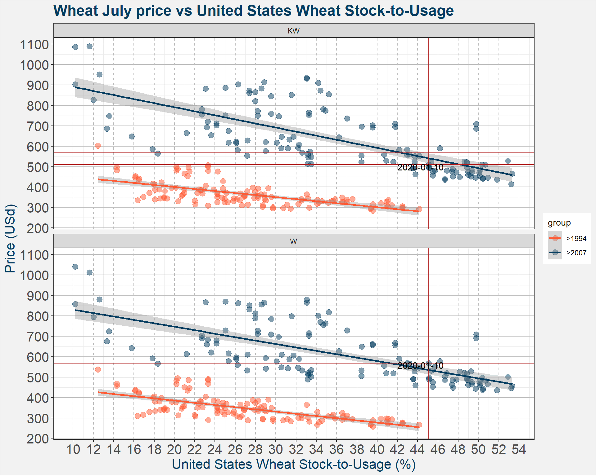
The images below give a graphical representation of the data. The x- and y-axes represent the Stock-to-Usage and Price of the July contract respectively.
From the images we can distinguish between two different regimes roughly corresponding to before and after 2007. This can be seen by the clear separation of the different coloured points in the plot below. The reason for this split is due to the broken Chicago Wheat contract where near dated futures prices stopped to converge to spot. Commercial grain users complained that this made it impossible to use the contract as a hedge. In an effor tto rectify the divergence in price the CME made changes including higher storage rates and more delivery points. This implies that the US wheat market before and after 2007 is fundamentaly different.
2 Deterministic Model
From the bubble chart above it looks like a linear model should be sufficient to model the July Wheat price as a function of stock-to-usage. Here we look at a couple slight modifications to improve upon the simple linear model.
We see that the prices are decreasing at a slower rate with increasing stock-to-usage numbers. Linear models on the other hand assume a constant rate of decrease. Here we look at two alternative models, a power-law and exponential model, both of which have decreasing rates of change.
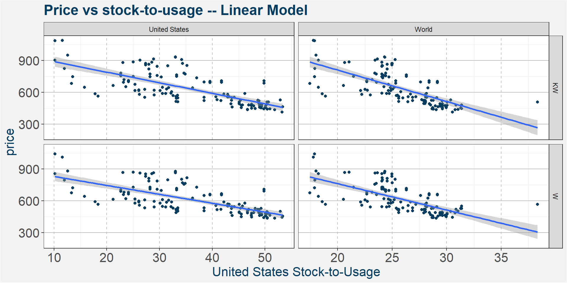
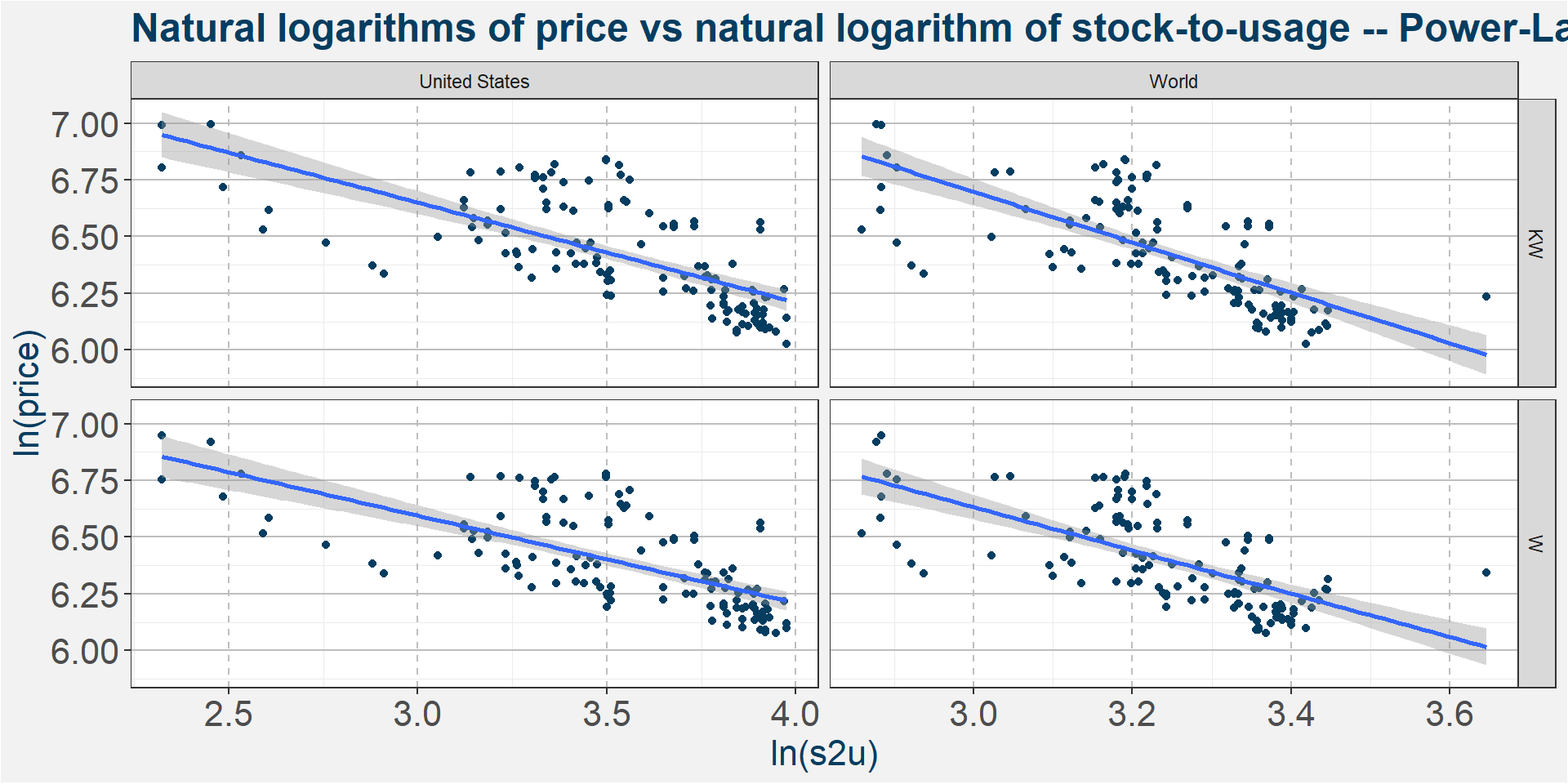
To find the best model it amounts to looking at the three different graphs below and deciding which has the best linear fit to the data. The equation describing the models are given below
Linear: \[ y = x \times m + c \]
Power-Law: \[ y = x^{m} \times \exp\left(c\right) \]
Exponential: \[ y = \exp\left( x \times m + c \right) \] In all three equations above \(x\) and \(y\) represent stock-to-usage and price respectively.
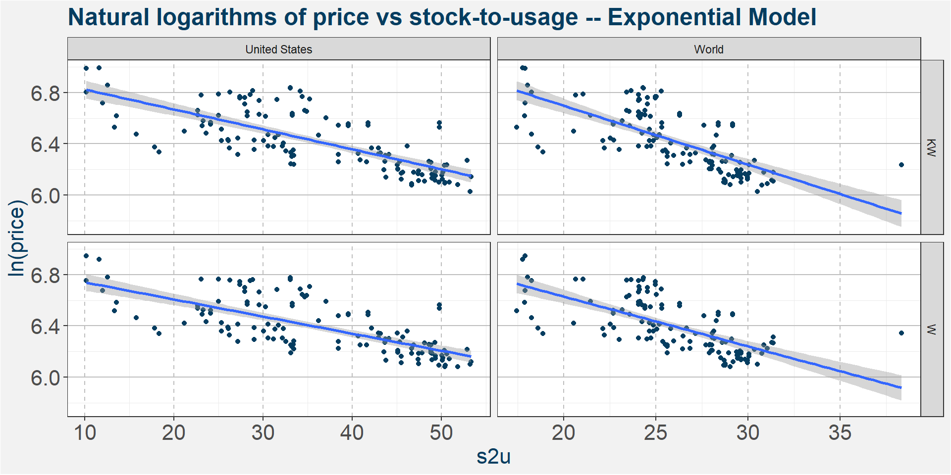
The plots below summarises the results of the model fitting. Each facet shows the R-squared value of the best fit for each commodity and contract code using the variable shown. In most of the cases the best fit model was the power-law. Notice that US wheat, crude and the dollar index made for the best fits for both Chicago and Kansas City wheat.
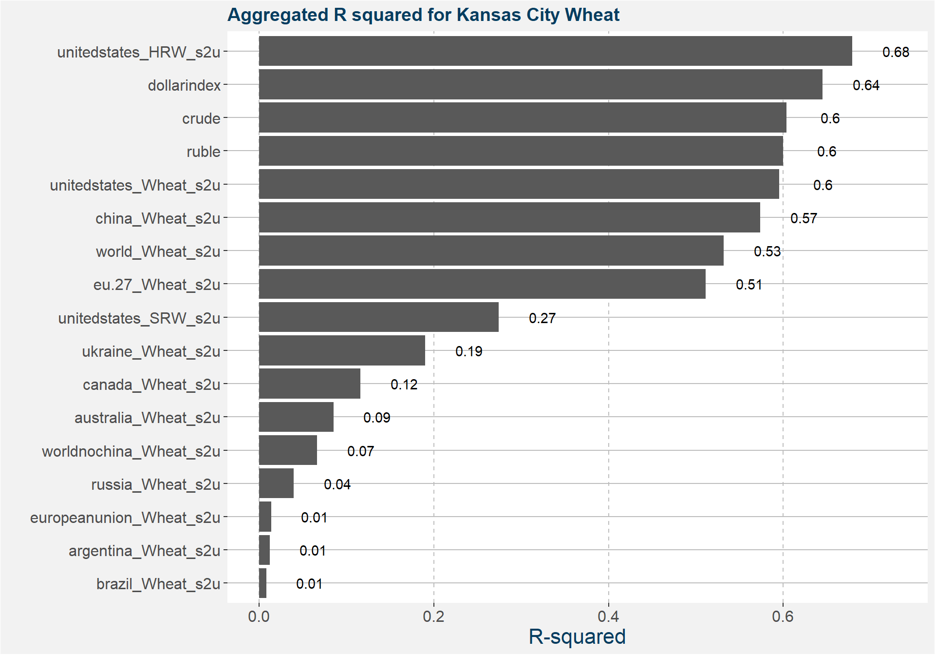
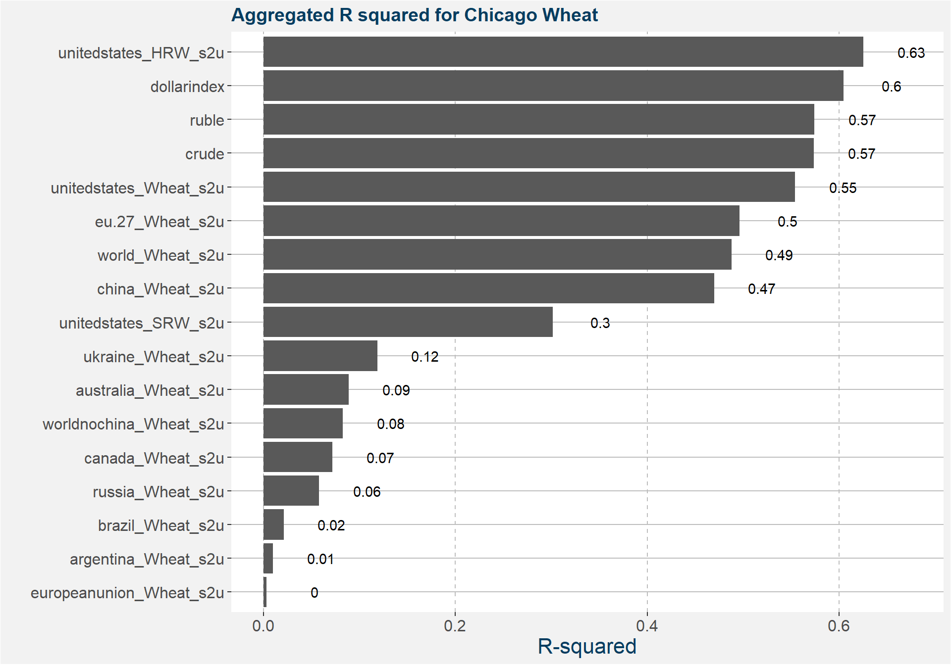
The table below summarises the results of the model fitting. Each cell shows the R-squared value of the fit for Kansas City Wheat. The models with the greatest R-squared values are shown at the top. From this naive in-sampe point of view we can see that crude is the best predictor followed in turn by the dollar index, Chinese and US stock-to-usages. In the following we have a closer look at the relationship between price and the main predictive features according to the table below.
| variable | exponential | linear | power law |
|---|---|---|---|
| dollarindex | 0.6421116 | 0.5908147 | 0.6436643 |
| ruble | 0.5849373 | 0.5305763 | 0.5944440 |
| china_Wheat_s2u | 0.5565902 | 0.5151923 | 0.5887901 |
| crude | 0.6070439 | 0.5725730 | 0.5877646 |
| unitedstates_HRW_s2u | 0.6341299 | 0.5850398 | 0.5848397 |
| unitedstates_Wheat_s2u | 0.5493019 | 0.5161688 | 0.4894438 |
| world_Wheat_s2u | 0.5033678 | 0.4787492 | 0.4819181 |
| eu.27_Wheat_s2u | 0.5009876 | 0.4419424 | 0.4719685 |
| unitedstates_SRW_s2u | 0.1879965 | 0.1773042 | 0.2220198 |
| ukraine_Wheat_s2u | 0.1348011 | 0.1065248 | 0.1936856 |
| canada_Wheat_s2u | 0.0944650 | 0.0688293 | 0.1186873 |
| australia_Wheat_s2u | 0.0531392 | 0.0602634 | 0.0359897 |
| worldnochina_Wheat_s2u | 0.0327006 | 0.0430374 | 0.0357462 |
| russia_Wheat_s2u | 0.0095849 | 0.0116085 | 0.0147158 |
| europeanunion_Wheat_s2u | 0.0063919 | 0.0031543 | 0.0119852 |
| brazil_Wheat_s2u | 0.0074155 | 0.0068554 | 0.0096433 |
| argentina_Wheat_s2u | 0.0013471 | 0.0000697 | 0.0069873 |
2.1 Deterministic Model Sensitivity
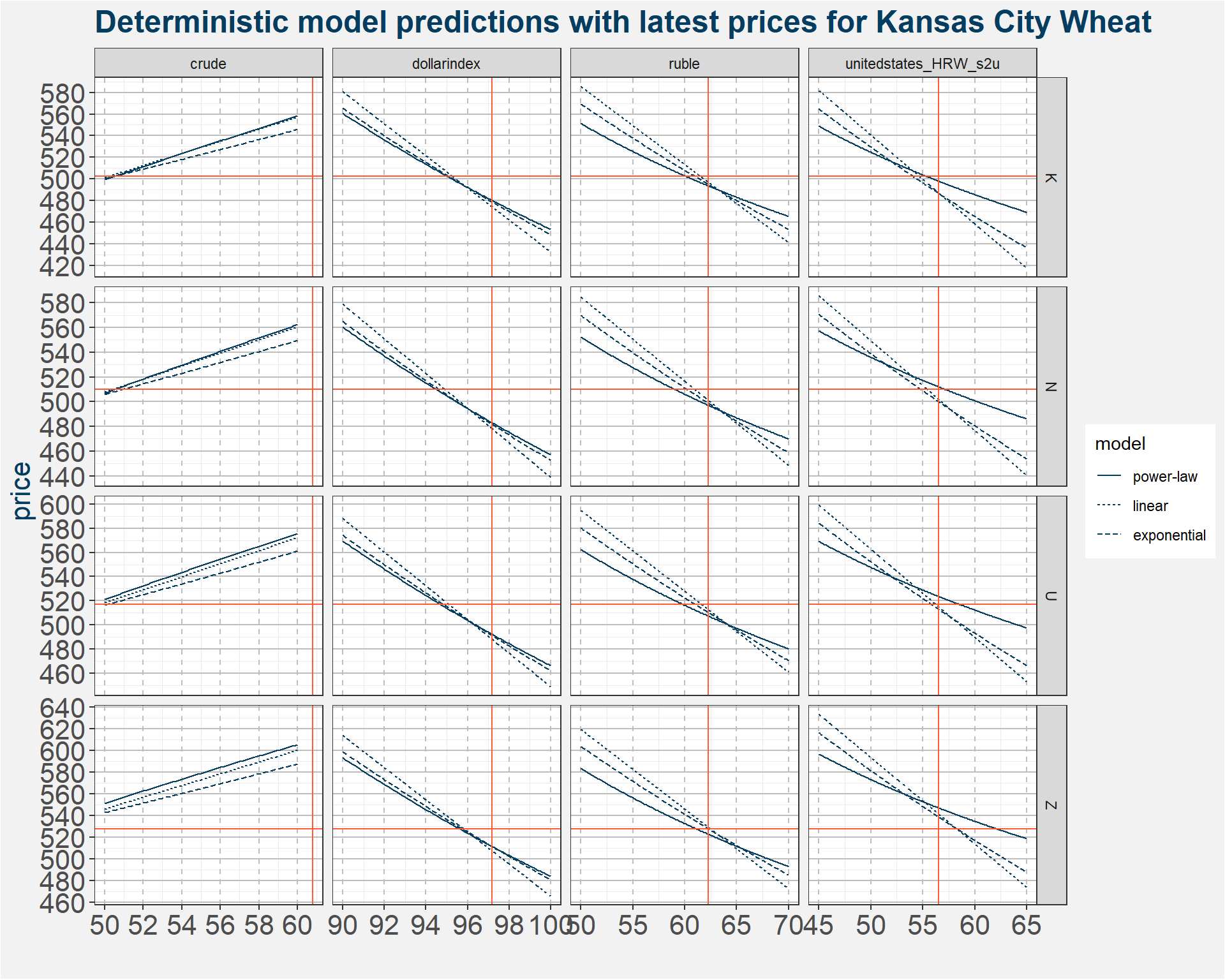
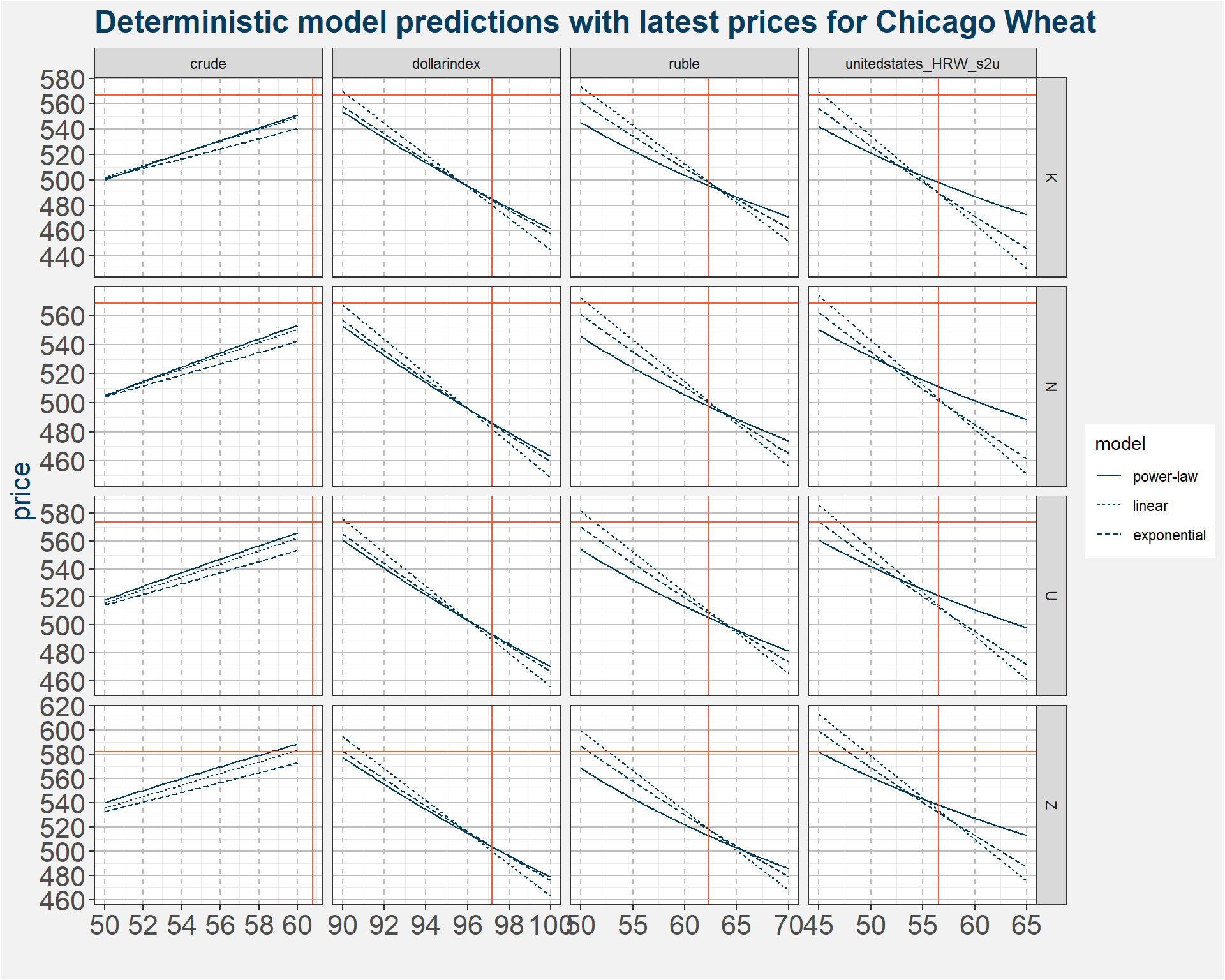
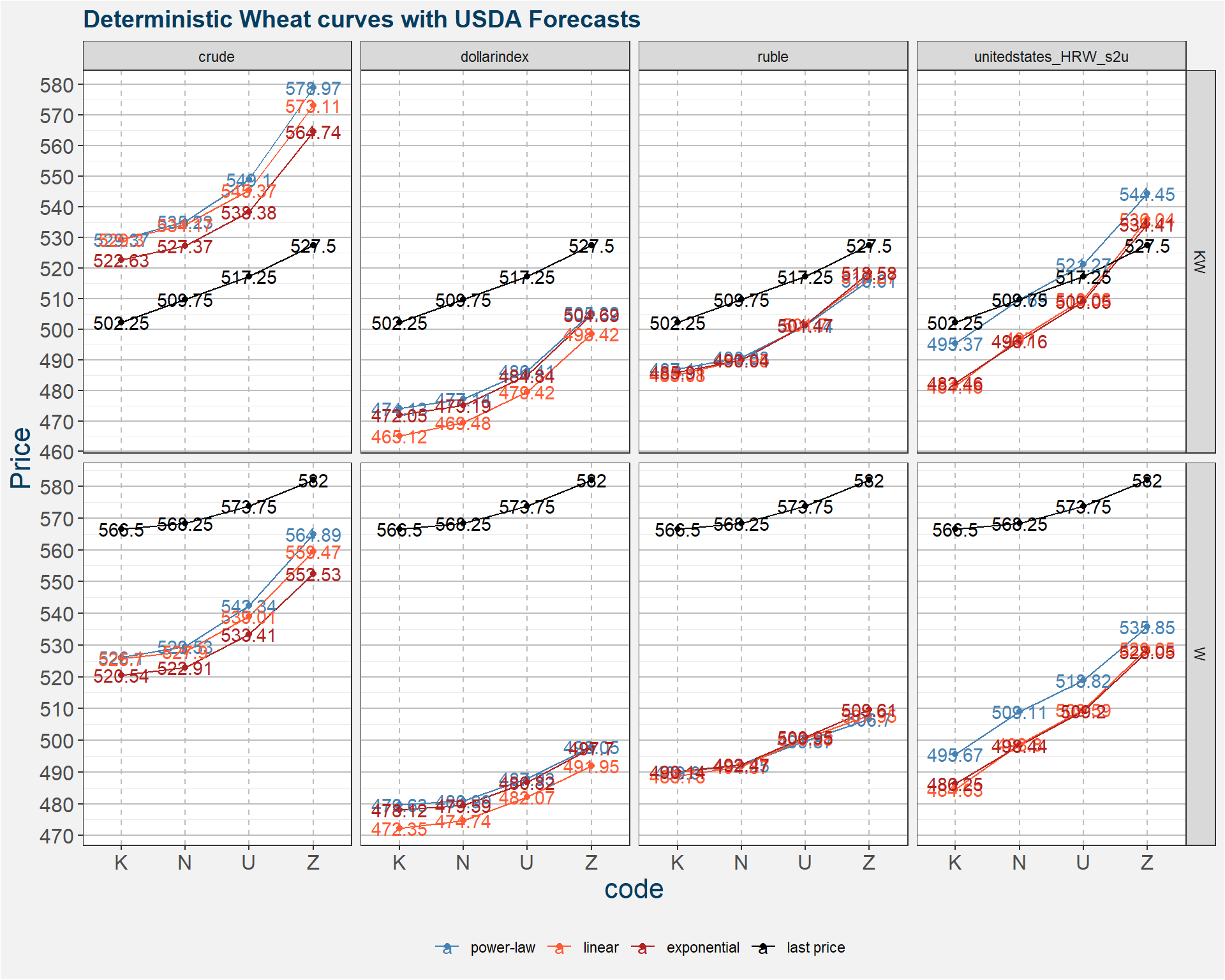
Taking the values from the table above we plot the model predictions in blue. The latest USDA United States stock-to-usage is given by the vertical orange line. The horizontal orange line gives the latest wheat N prices. The results can be interpreted in two ways. If we take the USDA numbers as the truth we need to see a downward adjustment in price. On the other hand we can imply a stock-to-usage from the latest price. Currently this number is much less than that reported by the USDA.
2.2 Deterministic Curve Prediction
3 Probabilistic Model
If we discretise the stock-to-usage percentages we are able to do some statistics on the values of the prices given stock-to-usage (or any other feature) in the discretised basket. In this way we can perform Bayesian statistics on the prices, i.e. given a forcast on the stock-to-usage we can determine the probability that the price is contained withing some interval.
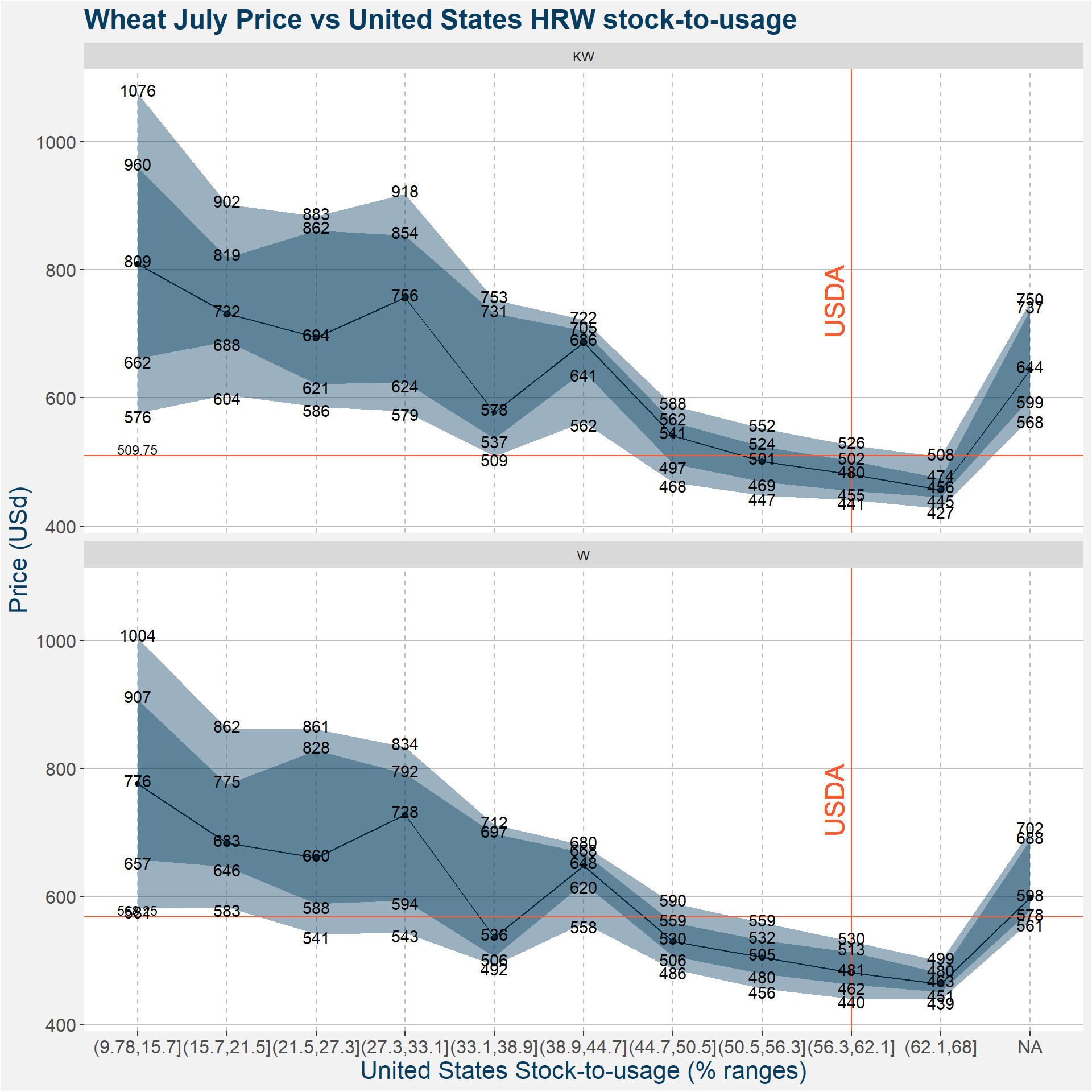
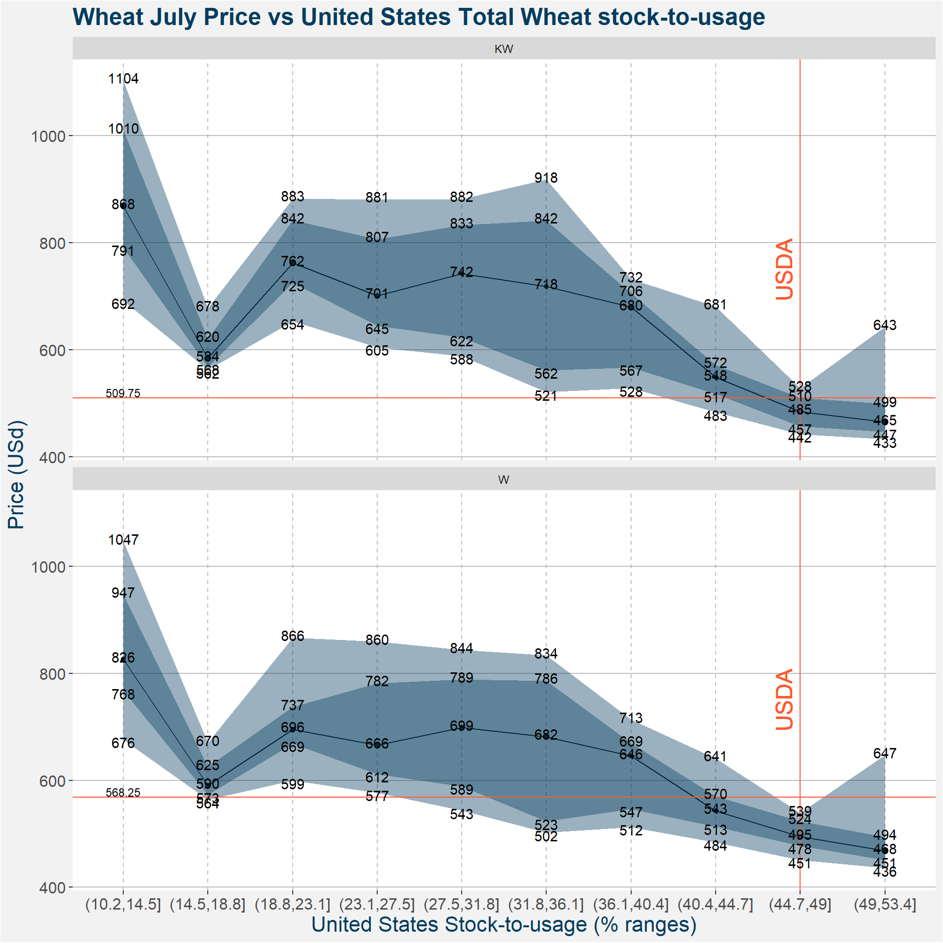
In the subsections below we show plots of the price statistics when the value of the underlyiing feature falls within the bucket specified on the x-axis. The solid black line shows the median price. The light and dark shaded regions show the 10th to 90th and 25th to 75th percentiles. The fat of the distributions lie withing the dark shaded region. For reference we also show the USDA and Polar Star fundamental forecast together with the latest price data. These are represented by the vertical and horizontal lines respectively. The same data used to create the images is also given in tabular form below the plots.
3.1 United States HRW Stock-to-Usage
| p10 | p25 | p50 | p75 | |
|---|---|---|---|---|
| (9.78,15.7] KW | 576.000 | 661.6250 | 809.375 | 959.8750 |
| (15.7,21.5] KW | 604.500 | 688.3750 | 731.500 | 818.8750 |
| (21.5,27.3] KW | 586.000 | 621.4375 | 694.000 | 861.7500 |
| (27.3,33.1] KW | 579.350 | 624.3750 | 756.250 | 853.5000 |
| (33.1,38.9] KW | 508.750 | 536.7500 | 577.625 | 731.3125 |
| (38.9,44.7] KW | 562.250 | 641.0625 | 686.500 | 705.0000 |
| (44.7,50.5] KW | 468.000 | 497.0000 | 540.750 | 562.5000 |
| (50.5,56.3] KW | 447.450 | 469.3125 | 501.125 | 524.0000 |
| (56.3,62.1] KW | 440.750 | 454.7500 | 480.250 | 501.5000 |
| (62.1,68] KW | 427.100 | 444.7500 | 456.375 | 474.0000 |
| NA KW | 568.100 | 599.0000 | 644.000 | 737.2500 |
| (9.78,15.7] W | 581.250 | 657.3750 | 775.750 | 907.1250 |
| (15.7,21.5] W | 583.250 | 646.5000 | 683.250 | 775.1250 |
| (21.5,27.3] W | 541.375 | 588.1875 | 660.250 | 828.4375 |
| (27.3,33.1] W | 543.350 | 594.1250 | 728.250 | 791.5000 |
| (33.1,38.9] W | 492.500 | 506.0000 | 536.125 | 697.4375 |
| (38.9,44.7] W | 558.375 | 620.0625 | 648.375 | 668.1875 |
| (44.7,50.5] W | 486.250 | 506.5000 | 529.750 | 558.7500 |
| (50.5,56.3] W | 455.725 | 479.5000 | 504.875 | 531.6250 |
| (56.3,62.1] W | 440.300 | 462.2500 | 481.250 | 513.0000 |
| (62.1,68] W | 439.150 | 450.8125 | 463.250 | 479.9375 |
| NA W | 560.750 | 577.5000 | 598.000 | 687.7500 |
3.2 United States Total Wheat Stock-to-Usage
| p10 | p25 | p50 | p75 | |
|---|---|---|---|---|
| (10.2,14.5] KW | 692.000 | 791.3125 | 868.500 | 1010.2500 |
| (14.5,18.8] KW | 562.000 | 568.0000 | 584.250 | 620.2500 |
| (18.8,23.1] KW | 653.525 | 725.2500 | 762.250 | 842.2500 |
| (23.1,27.5] KW | 604.875 | 645.4375 | 701.250 | 806.7500 |
| (27.5,31.8] KW | 588.250 | 622.5000 | 742.250 | 832.7500 |
| (31.8,36.1] KW | 520.700 | 561.8750 | 718.500 | 841.8750 |
| (36.1,40.4] KW | 528.300 | 567.1250 | 679.750 | 705.8750 |
| (40.4,44.7] KW | 483.250 | 517.4375 | 548.250 | 571.8750 |
| (44.7,49] KW | 442.500 | 456.7500 | 484.750 | 509.7500 |
| (49,53.4] KW | 432.650 | 446.7500 | 465.000 | 498.7500 |
| (10.2,14.5] W | 676.300 | 767.6250 | 826.500 | 946.9375 |
| (14.5,18.8] W | 563.750 | 572.6250 | 590.500 | 624.9375 |
| (18.8,23.1] W | 599.400 | 668.5625 | 695.500 | 737.1250 |
| (23.1,27.5] W | 577.000 | 611.8125 | 665.625 | 781.8750 |
| (27.5,31.8] W | 543.250 | 589.0000 | 698.750 | 788.6250 |
| (31.8,36.1] W | 501.950 | 523.1250 | 681.750 | 786.2500 |
| (36.1,40.4] W | 512.500 | 546.6250 | 645.500 | 669.2500 |
| (40.4,44.7] W | 484.250 | 513.4375 | 543.125 | 570.3750 |
| (44.7,49] W | 451.250 | 478.0000 | 495.000 | 523.7500 |
| (49,53.4] W | 436.150 | 451.0000 | 468.250 | 494.2500 |
3.3 World Stock-to-Usage
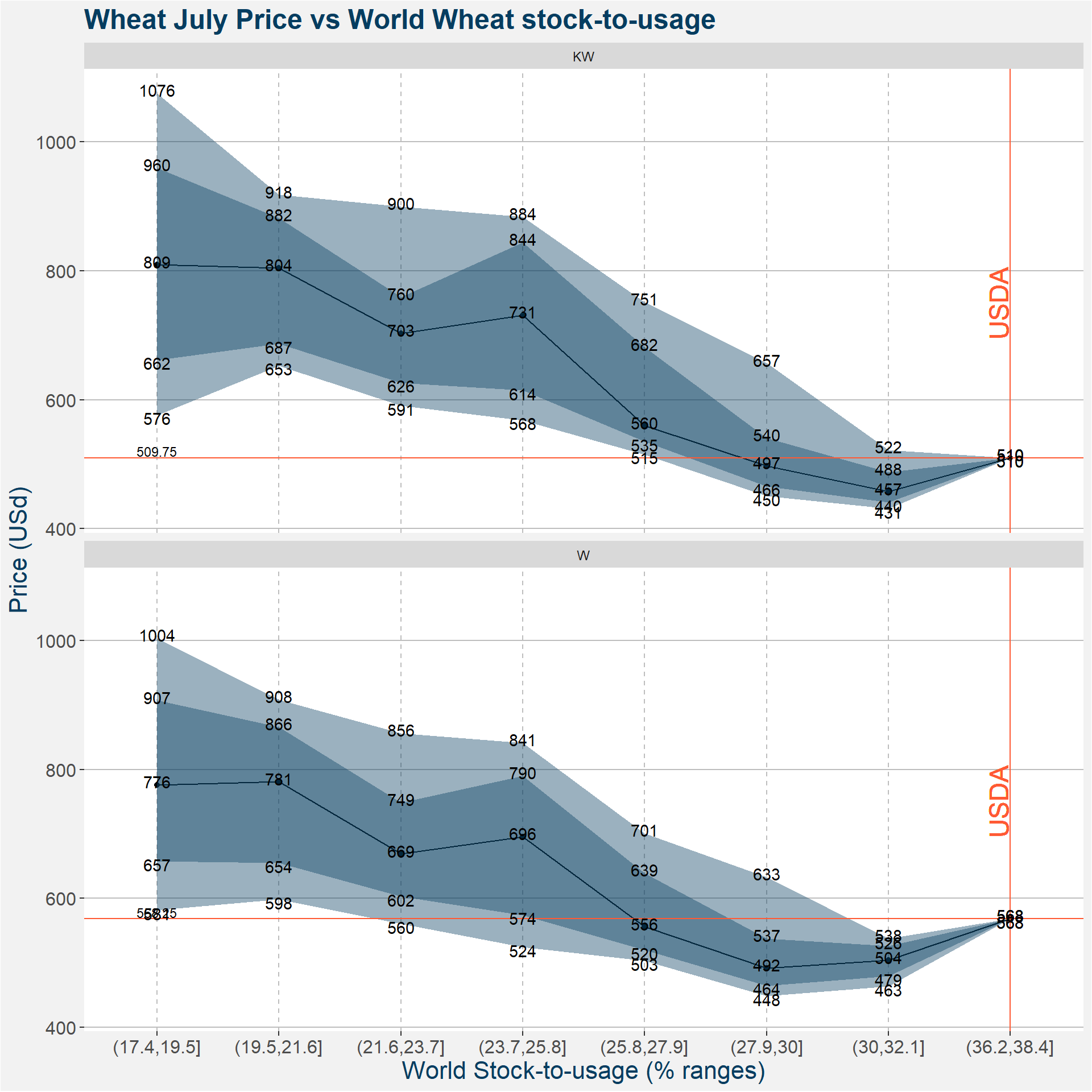
| p10 | p25 | p50 | p75 | |
|---|---|---|---|---|
| (17.4,19.5] KW | 576.00 | 661.625 | 809.375 | 959.875 |
| (19.5,21.6] KW | 652.75 | 687.000 | 804.500 | 882.000 |
| (21.6,23.7] KW | 590.75 | 626.250 | 703.250 | 759.625 |
| (23.7,25.8] KW | 568.00 | 614.500 | 731.000 | 844.000 |
| (25.8,27.9] KW | 515.10 | 535.250 | 559.500 | 681.500 |
| (27.9,30] KW | 450.00 | 465.625 | 497.250 | 540.500 |
| (30,32.1] KW | 430.95 | 440.500 | 457.250 | 487.750 |
| (36.2,38.4] KW | 509.75 | 509.750 | 509.750 | 509.750 |
| (17.4,19.5] W | 581.25 | 657.375 | 775.750 | 907.125 |
| (19.5,21.6] W | 598.00 | 654.500 | 780.750 | 865.750 |
| (21.6,23.7] W | 560.05 | 602.500 | 668.750 | 748.875 |
| (23.7,25.8] W | 524.00 | 574.000 | 695.500 | 790.000 |
| (25.8,27.9] W | 503.15 | 519.875 | 555.750 | 639.375 |
| (27.9,30] W | 448.30 | 464.375 | 492.000 | 537.375 |
| (30,32.1] W | 463.45 | 479.000 | 503.750 | 526.000 |
| (36.2,38.4] W | 568.25 | 568.250 | 568.250 | 568.250 |
3.4 World Stock-to-Usage without China
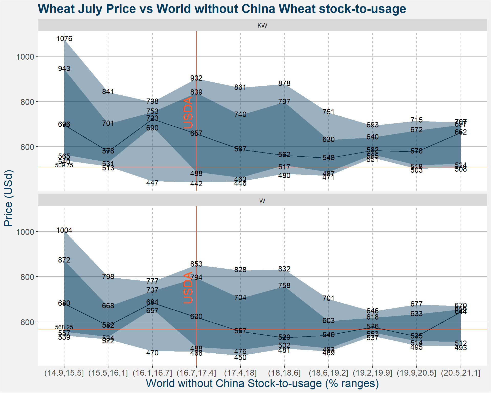
| p10 | p25 | p50 | p75 | |
|---|---|---|---|---|
| (14.9,15.5] KW | 540.000 | 564.5625 | 696.125 | 943.1250 |
| (15.5,16.1] KW | 513.025 | 531.1875 | 578.375 | 700.7500 |
| (16.1,16.7] KW | 446.525 | 690.0000 | 722.875 | 753.3125 |
| (16.7,17.4] KW | 442.300 | 488.2500 | 656.750 | 838.6250 |
| (17.4,18] KW | 445.500 | 462.5625 | 587.125 | 740.0000 |
| (18,18.6] KW | 479.525 | 517.2500 | 562.000 | 797.1250 |
| (18.6,19.2] KW | 470.725 | 487.1875 | 548.500 | 629.5625 |
| (19.2,19.9] KW | 551.100 | 565.2500 | 582.500 | 640.5000 |
| (19.9,20.5] KW | 503.000 | 518.4375 | 577.750 | 671.9375 |
| (20.5,21.1] KW | 507.500 | 524.0000 | 662.000 | 696.7500 |
| (14.9,15.5] W | 539.000 | 556.8750 | 680.000 | 871.6875 |
| (15.5,16.1] W | 522.400 | 534.0000 | 582.250 | 668.1875 |
| (16.1,16.7] W | 469.925 | 657.0625 | 684.500 | 737.0625 |
| (16.7,17.4] W | 468.400 | 488.3750 | 620.250 | 794.0000 |
| (17.4,18] W | 449.525 | 475.5625 | 557.125 | 704.2500 |
| (18,18.6] W | 481.350 | 502.0625 | 529.000 | 757.5625 |
| (18.6,19.2] W | 469.450 | 483.0625 | 540.125 | 602.9375 |
| (19.2,19.9] W | 537.100 | 553.2500 | 576.500 | 618.2500 |
| (19.9,20.5] W | 494.800 | 514.3750 | 534.750 | 633.2500 |
| (20.5,21.1] W | 492.750 | 512.0000 | 643.500 | 655.5000 |
3.5 Mean Crude
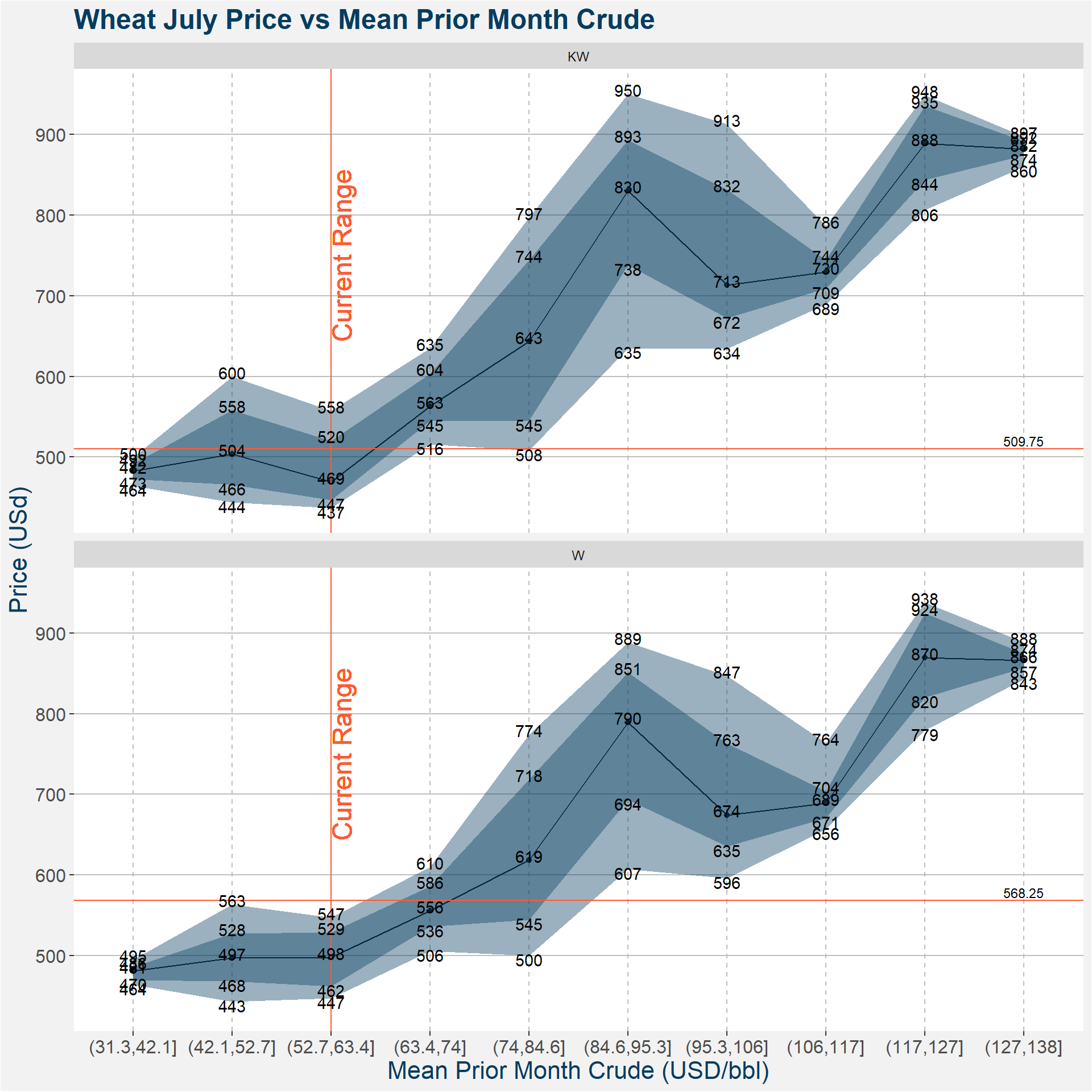
| p10 | p25 | p50 | p75 | |
|---|---|---|---|---|
| (31.3,42.1] KW | 464.500 | 472.8125 | 482.500 | 491.6875 |
| (42.1,52.7] KW | 444.075 | 465.8750 | 503.625 | 558.2500 |
| (52.7,63.4] KW | 437.000 | 446.9375 | 469.125 | 520.2500 |
| (63.4,74] KW | 515.650 | 544.7500 | 563.000 | 603.5000 |
| (74,84.6] KW | 508.200 | 545.0000 | 643.250 | 744.5000 |
| (84.6,95.3] KW | 634.750 | 737.8125 | 830.250 | 893.3125 |
| (95.3,106] KW | 634.300 | 672.2500 | 713.250 | 831.7500 |
| (106,117] KW | 689.000 | 709.0000 | 729.500 | 744.5000 |
| (117,127] KW | 806.025 | 843.6875 | 888.500 | 935.3750 |
| (127,138] KW | 860.000 | 874.2500 | 882.000 | 891.5000 |
| (31.3,42.1] W | 463.825 | 469.9375 | 480.625 | 485.7500 |
| (42.1,52.7] W | 442.975 | 468.3750 | 497.000 | 527.6875 |
| (52.7,63.4] W | 446.800 | 462.1875 | 497.875 | 528.8125 |
| (63.4,74] W | 505.550 | 536.2500 | 555.500 | 585.7500 |
| (74,84.6] W | 500.150 | 544.7500 | 618.750 | 718.5000 |
| (84.6,95.3] W | 607.275 | 693.5000 | 789.500 | 851.3125 |
| (95.3,106] W | 595.750 | 635.1250 | 674.500 | 763.0000 |
| (106,117] W | 656.500 | 670.7500 | 688.750 | 703.7500 |
| (117,127] W | 779.000 | 820.3125 | 869.625 | 924.3125 |
| (127,138] W | 842.850 | 856.8750 | 865.750 | 874.2500 |
3.6 Dollar Index
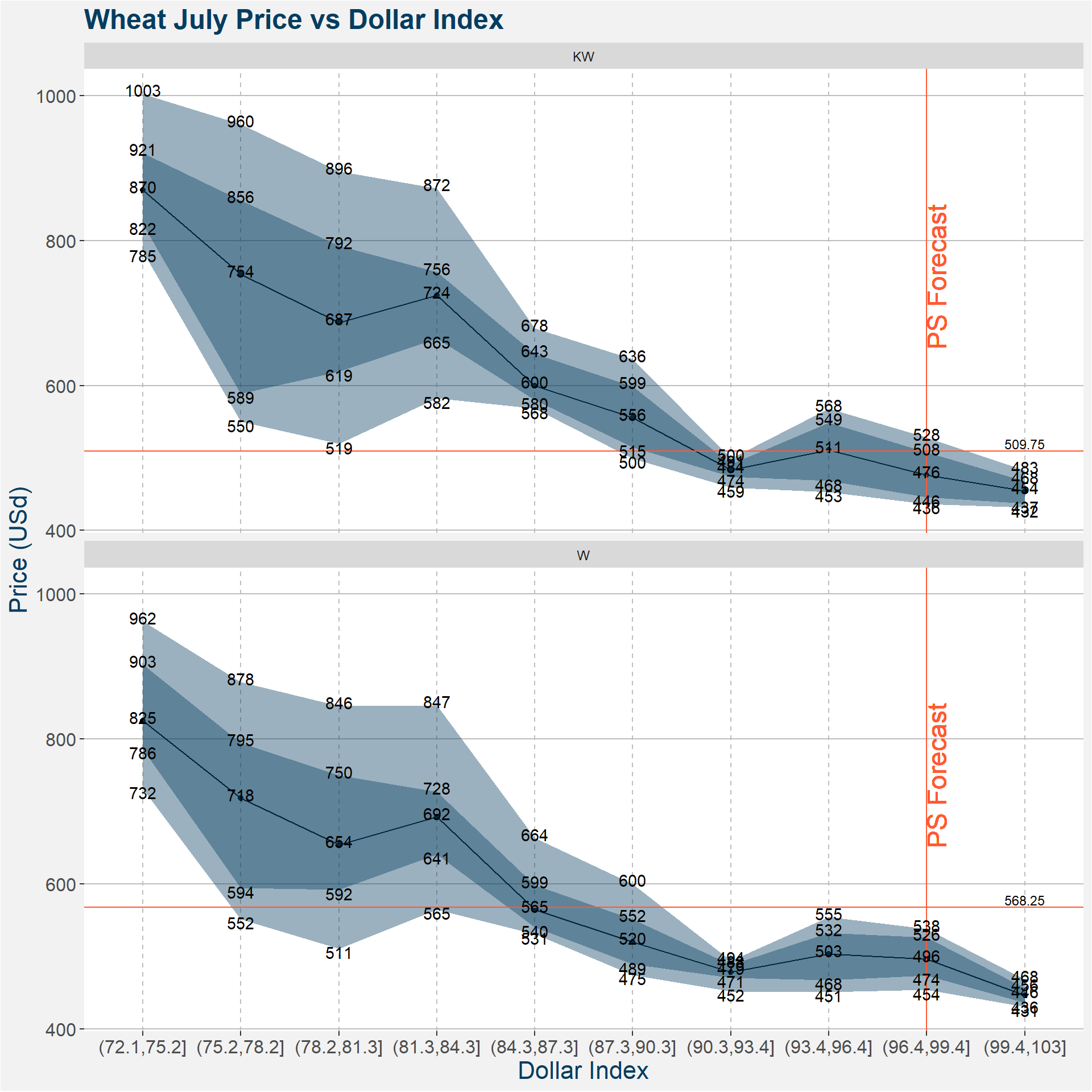
| p10 | p25 | p50 | p75 | |
|---|---|---|---|---|
| (72.1,75.2] KW | 784.600 | 822.3125 | 869.500 | 920.7500 |
| (75.2,78.2] KW | 550.000 | 588.8750 | 753.500 | 855.7500 |
| (78.2,81.3] KW | 519.250 | 619.3750 | 687.000 | 792.5000 |
| (81.3,84.3] KW | 582.000 | 664.7500 | 724.250 | 756.2500 |
| (84.3,87.3] KW | 568.000 | 580.0625 | 599.750 | 643.4375 |
| (87.3,90.3] KW | 499.500 | 515.0000 | 555.750 | 599.0000 |
| (90.3,93.4] KW | 459.475 | 474.3750 | 483.500 | 491.0000 |
| (93.4,96.4] KW | 453.200 | 468.2500 | 510.750 | 548.7500 |
| (96.4,99.4] KW | 436.300 | 446.1250 | 476.500 | 507.7500 |
| (99.4,103] KW | 432.000 | 437.3750 | 454.500 | 468.0000 |
| (72.1,75.2] W | 731.550 | 786.3125 | 825.250 | 902.8125 |
| (75.2,78.2] W | 551.500 | 594.3750 | 718.250 | 794.6250 |
| (78.2,81.3] W | 511.000 | 592.0000 | 654.250 | 749.8750 |
| (81.3,84.3] W | 565.100 | 641.0000 | 692.500 | 727.5000 |
| (84.3,87.3] W | 530.875 | 540.3750 | 564.625 | 598.5625 |
| (87.3,90.3] W | 474.750 | 489.2500 | 520.250 | 551.7500 |
| (90.3,93.4] W | 451.925 | 470.9375 | 478.750 | 488.3750 |
| (93.4,96.4] W | 450.950 | 467.5000 | 503.250 | 532.5000 |
| (96.4,99.4] W | 453.950 | 473.8750 | 496.500 | 526.3750 |
| (99.4,103] W | 430.650 | 436.0000 | 446.500 | 456.2500 |
3.7 Ruble
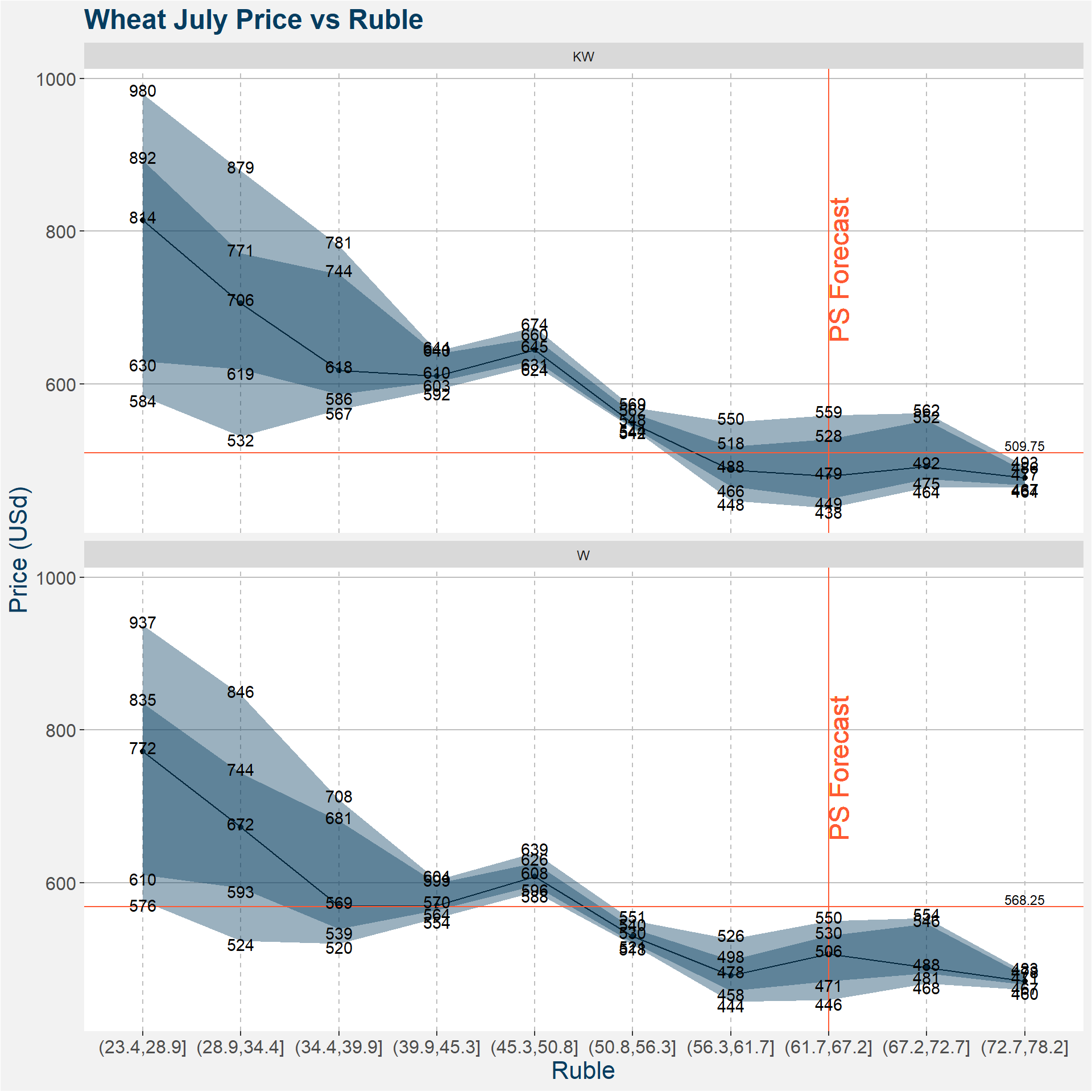
| p10 | p25 | p50 | p75 | |
|---|---|---|---|---|
| (23.4,28.9] KW | 583.650 | 630.0000 | 814.250 | 892.5000 |
| (28.9,34.4] KW | 531.625 | 619.0625 | 705.625 | 771.0000 |
| (34.4,39.9] KW | 566.650 | 586.3750 | 617.750 | 744.0000 |
| (39.9,45.3] KW | 592.500 | 603.2500 | 610.250 | 639.7500 |
| (45.3,50.8] KW | 624.250 | 631.2500 | 644.750 | 660.5000 |
| (50.8,56.3] KW | 541.625 | 543.5000 | 548.375 | 561.6875 |
| (56.3,61.7] KW | 447.500 | 465.8750 | 487.750 | 518.0000 |
| (61.7,67.2] KW | 437.500 | 449.0625 | 479.000 | 527.5000 |
| (67.2,72.7] KW | 464.275 | 475.2500 | 491.750 | 552.1250 |
| (72.7,78.2] KW | 464.500 | 467.1250 | 477.000 | 486.1250 |
| (23.4,28.9] W | 575.650 | 609.7500 | 772.000 | 835.0000 |
| (28.9,34.4] W | 523.975 | 593.2500 | 672.375 | 743.5000 |
| (34.4,39.9] W | 520.150 | 539.0000 | 569.000 | 680.6250 |
| (39.9,45.3] W | 553.500 | 564.0000 | 570.000 | 598.7500 |
| (45.3,50.8] W | 587.750 | 596.0000 | 608.000 | 626.0000 |
| (50.8,56.3] W | 518.225 | 521.3750 | 529.875 | 540.0625 |
| (56.3,61.7] W | 443.750 | 458.3750 | 478.500 | 498.3750 |
| (61.7,67.2] W | 446.250 | 470.5625 | 506.250 | 530.0000 |
| (67.2,72.7] W | 467.500 | 481.1875 | 488.375 | 545.7500 |
| (72.7,78.2] W | 459.850 | 466.6250 | 470.750 | 478.1250 |
4 Ensemble Model
We have created ensemble machine learning models that predict the wheat prices along the futures curve. These models take as inputs the stock-to-usage percentages of the top wheat producing and consuming nations together with the dollar index and month prior average crude price as proxies for the US Dollar and energy respectively.
The ensemble models we create are all random forest regression models. We create a train and test split and perform hyper parameter tuning on the training set using 3 fold cross-validation. Ensemble models are a natural extension of the single variable deterministic models in that they are able to gain from possible interactions between the different input features.
From the best models we determine the variable importance of all the input features. The results are sumarised in the plot below. The greater the importance the larger the effect of that feature on the predicted values. The most important feature for each of the two different classes of wheat and contract codes are highlighted in orange.
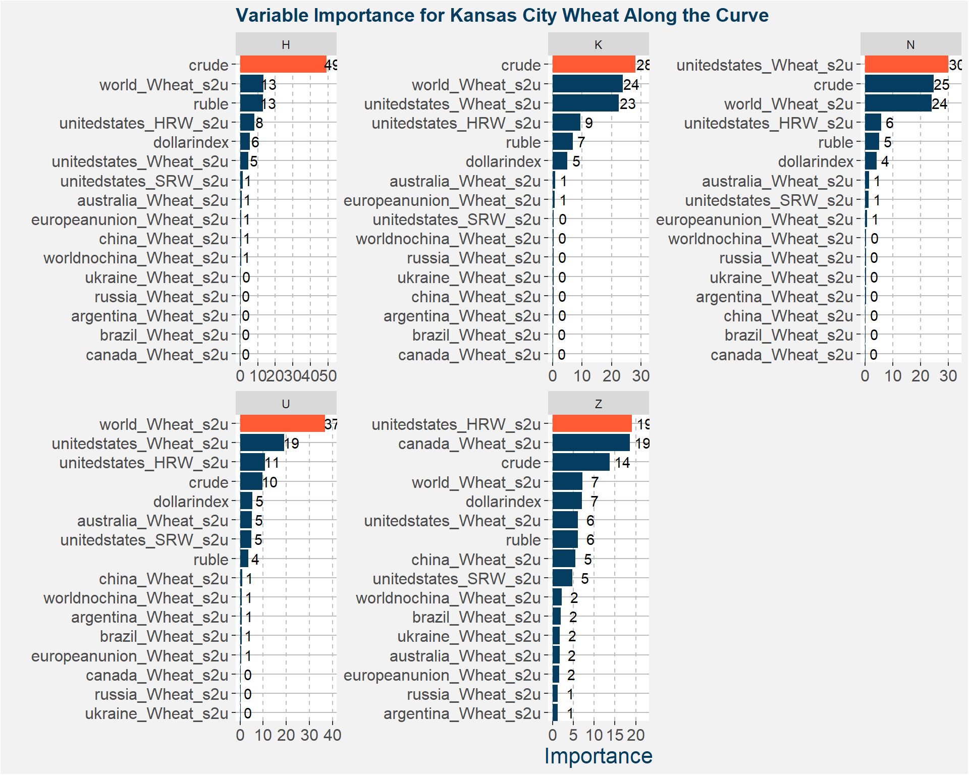
In the plot below we aggregate all the feature importances along the curve into a single representation.
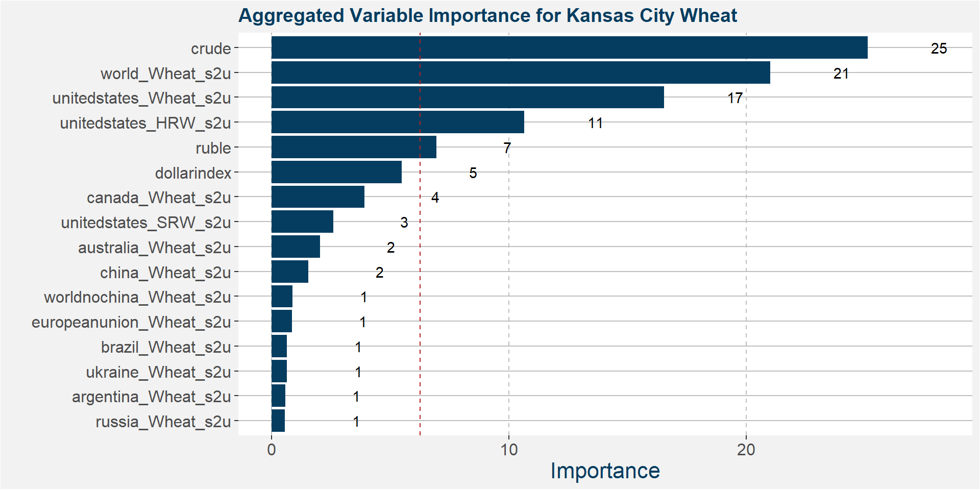
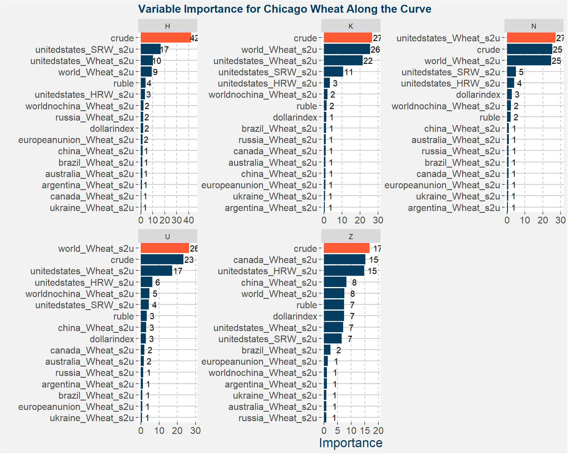
Similar to the Kansas City case, we aggregate all the feature importances along the curve into a single representation.
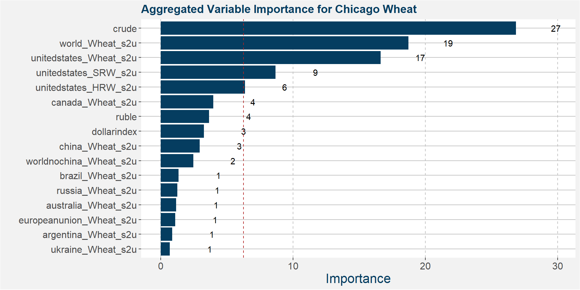
Notice that the features with greatest importance is crude, world wheat s2u and unitedstates_HRW_s2u. The table below gives the R-squared values of the ensemble models fitted to the data. Notice the significant improvement over the deterministic models.
| H | K | N | U | Z | |
|---|---|---|---|---|---|
| KW | 0.86 | 0.74 | 0.77 | 0.92 | 0.43 |
| W | 0.74 | 0.60 | 0.64 | 0.86 | 0.39 |
4.1 Crude Sensitivity
As the cost of energy increases we expect the price of wheat to increase. This intuition is confirmed in the plots below. The y-and x-axis show the prediction and value of crude respectively. Here we fix all parameters to the latest WASDE numbers, but allow the value of the prior month crude price the change from 40 to 80. In the plots below we see the monotonic increasing relationship between the two variables. We can also see an elbow forming at crude prices greater than 75.
4.2 United States HRW Stock-to-Usage Sensitivity
As the United States HRW Stock-to-Usage percentages increase we expect the price of wheat to decrease. This intuition is confirmed in the plots below. The y-and x-axis show the prediction and value of United States Stock-to-Usage respectively. Here we fix all parameters to the latest WASDE numbers, but allow the value of United States Stock-To-Usage the change from 45 to 65. In the plots below we see the quasi monotonic decreasing relationship between the two variables. We can also see transition values that resembles a phase transition for values of United States HRW Stock-to-Usage around 52.
4.3 World Stock-to-Usage Sensitivity
As the wolrd Stock-to-Usage percentages increase we expect the price of wheat to decrease. This intuition is confirmed in the plots below. The y-and x-axis show the prediction and value of world Stock-to-Usage respectively. Here we fix all parameters to the latest WASDE numbers, but allow the value of world Stock-To-Usage the change from 30 to 50. In the plots below we see the quasi monotonic decreasing relationship between the two variables. We can also see transition values that resembles a phase transition for values of world Stock-to-Usage around 25.
4.4 Ruble Sensitivity
5 Robust Model
The robust model is formed by only using the features with the greatest contribution in terms of feature importance. In this case we only use
- World Wheat stocks
- Total United States stock
- United States HRW stock
- Crude
- Ruble
Below we show the feature importances of these new models.
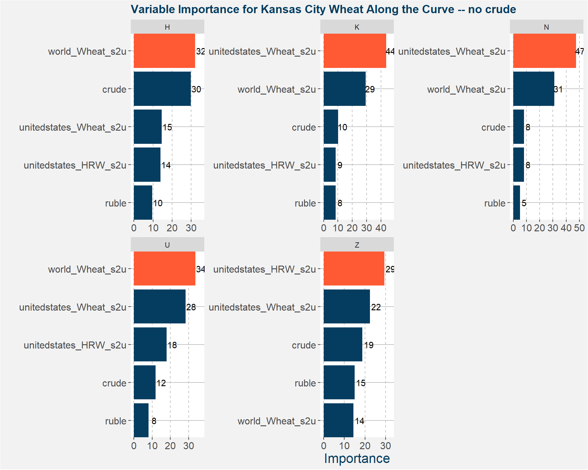
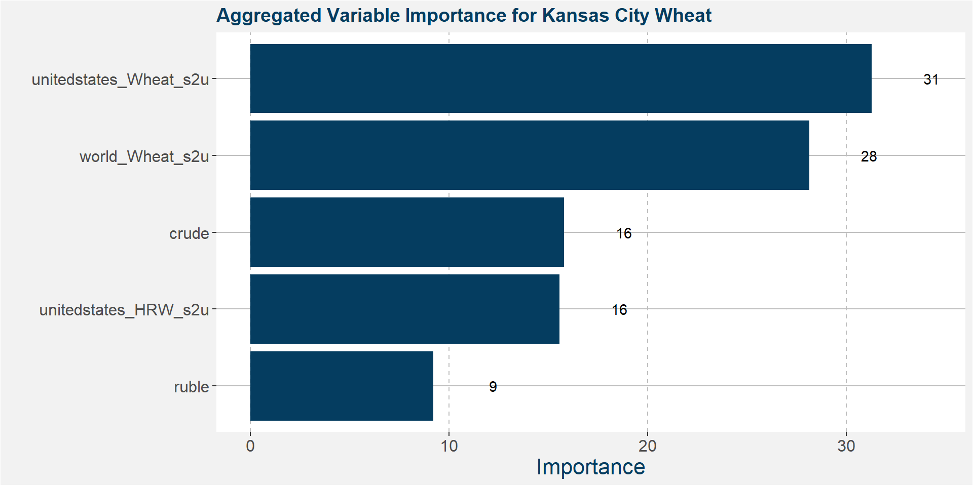
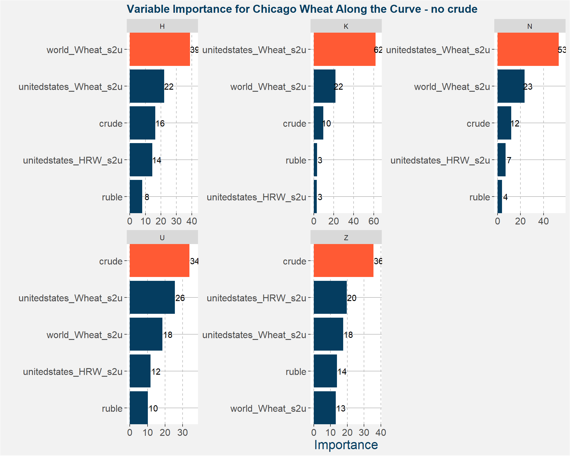
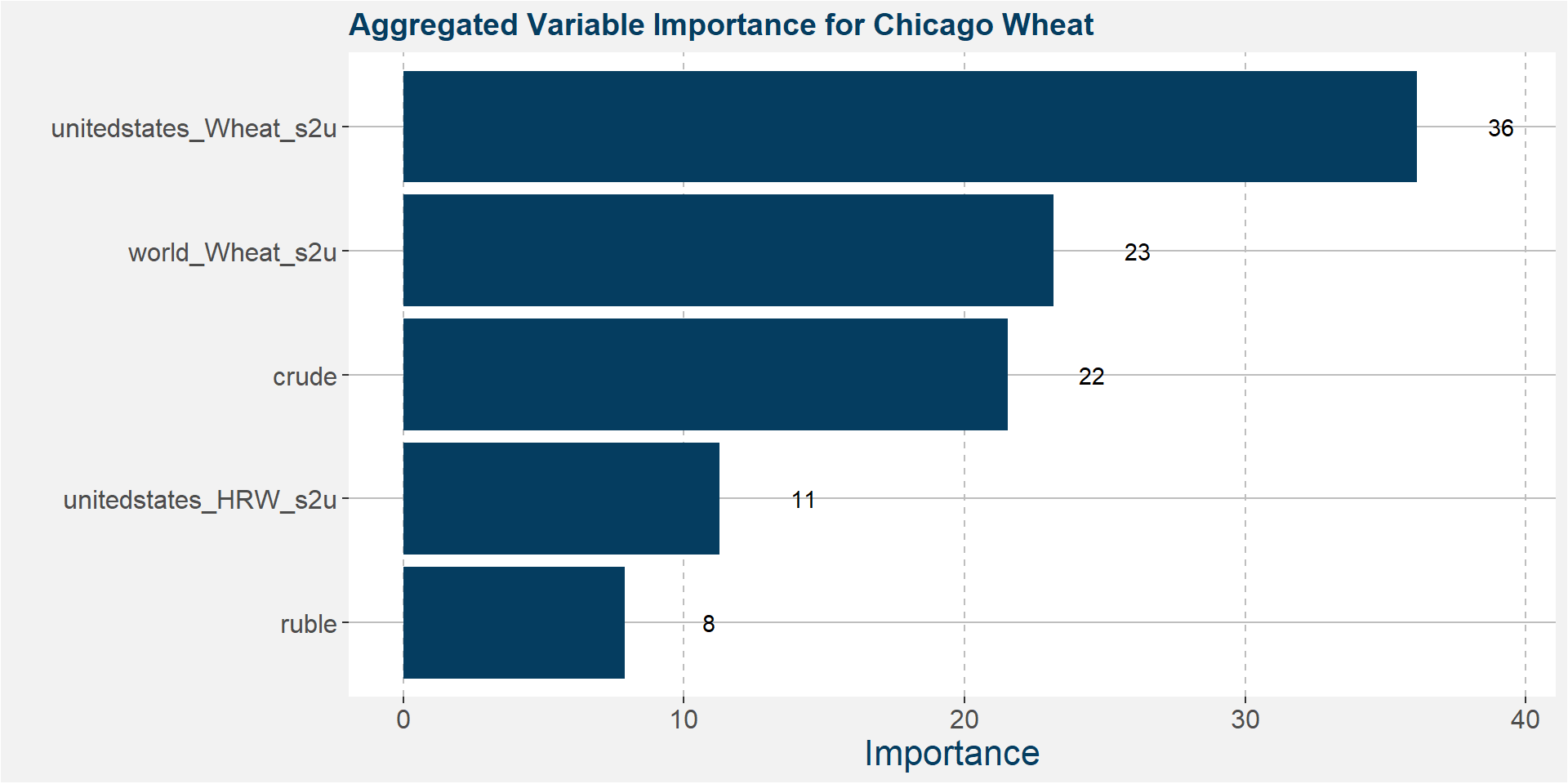
The table below shows the R-squared values of the models. Notice that the models that contain crude as a feature perform slighlty better than those without crude. Overall the results withour crude are still good.
| comdty | code | all features | reduced features |
|---|---|---|---|
| KW | H | 0.86 | 0.89 |
| KW | K | 0.74 | 0.67 |
| KW | N | 0.77 | 0.64 |
| KW | U | 0.92 | 0.93 |
| KW | Z | 0.43 | 0.21 |
| W | H | 0.74 | 0.72 |
| W | K | 0.60 | 0.08 |
| W | N | 0.64 | 0.17 |
| W | U | 0.86 | 0.89 |
| W | Z | 0.39 | 0.19 |
6 Predictions
The plot below shows the ensemble model predictions for USDA forecasted fundamentals. It is difficult to pin down the value of crude, so we consider a range of values form 50 to 60. Furthermore we consider all the predictions from each of the decision trees model to determine prediction statistics. The normal output of a collection of regression trees is the mean of all the predictions. In the plot below we sohw the 25th to 75th percentiles of the predicted prices, this corresponds to the area between the two gray curves. The latest price data is represented by the black curve. The median model prediction is shown in blue. here we use the median as it is les likely to be skewed by possible outliers. We also include the results for the model withour crude as a feature. Results are very similar.
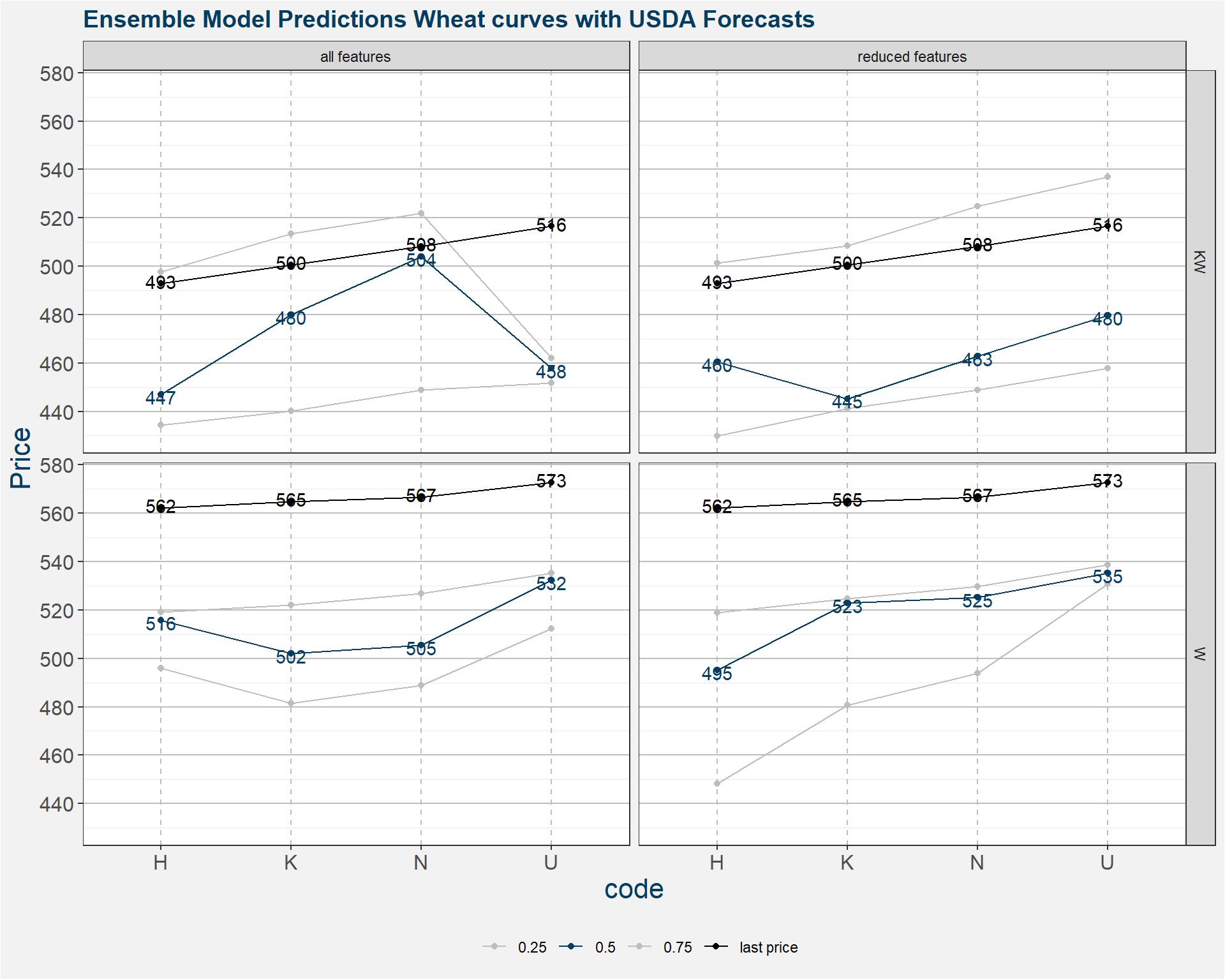
The image above shows that KW is withing the model predictions, however it is on the high end of the predictions. W on the other hand is well outside of the model predictions.