Introduction
In this post we indroduce another way to express a relative value trade between two different commodities. The main idea is to use a bullspread in one commodity and a bearspread in a closely related commodity. In this way we can use different calendar spreads to express our relative value point of view. This method is interesting because it enables us to use previous work on the modeling of calendar spreads using fundamental parameters to give possible ranges where the relative value spread should be given the underlying fundamentals.
Similar to the relative sizing of normal relative value trades we use the same sizing process for the long (bullspread) and short (bearspread) legs. Recall that our convention for normal relative value trades is to express the spread of commodity 1 vs commodity 2 as
\[ S = P_{\text{commodity 2}} -P_{\text{commodity 1}} \] where \(P_i\) denotes the price of \(i\). We use a similar methodology in the case of the relative calendars where we write
\[ S = S^{\text{commodity 2}}_{\text{calRef 2}} - S^{\text{commodity 1}}_{\text{calRef 1}} \] where \(S^{\text{commodity } i}_{\text{calRef } i}\) is the standard calendar spread definition of commodity \(i\) with calendar reference calRef \(i\). Recall we use the notation of front - deferred for the calendar spreads.
Similar to the case where the normal relative value rallies because of a rally in the price of commodity 2 we will see that the curve of commodity 2 should move in a direction of increased backwardation. In this case the relative calendar should also increase in value, but not to the same extent because of the way the trade is beying expressed.
Shiny
These results have been added to Shiny to a new tab called Relative Calendars. Currently we are still in a testing phase with only a collection of relative value pairs available. Below is a screenshot of what the current offereng looks like.
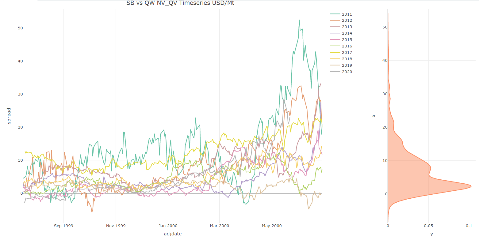
Similar to the other tabs we see a time series and corresponding distribution when a particular relative value pair is selected. Below we show the example of the SB vs QW NV_QV spread. A note on the notion used here, the NV spread is associated with the first commodity, in this case SB. The QC spread is associated with QW and the spread is calculated as
\[ S = S^{QW}_{QV} - S^{SB}_{NV} = ( P^{QW}_{Q} - P^{QW}_{V} ) - ( P^{SB}_{N} - P^{SB}_{V} ) \] where \(P^{a}_{b}\) denotes the price of \(a\) with contract code \(b\).
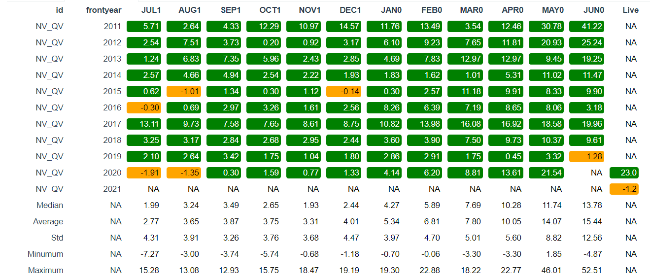
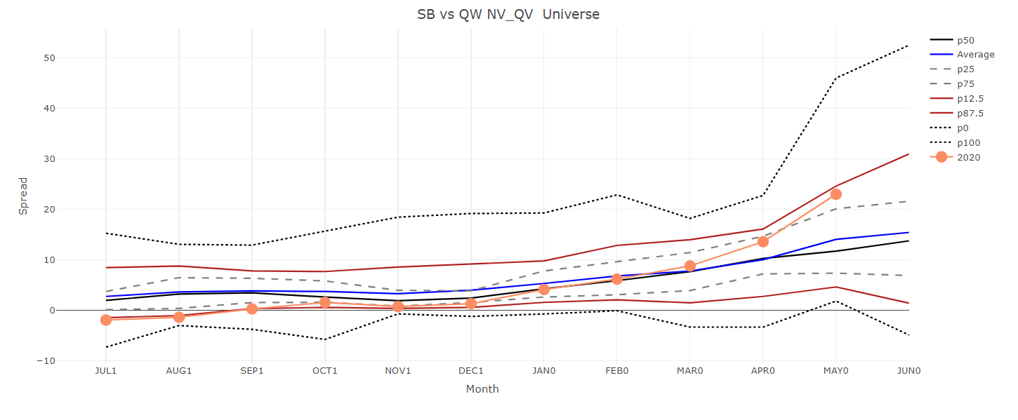
Similar to the other cases we summarize the data in tabular and graphical form for easy viewing.
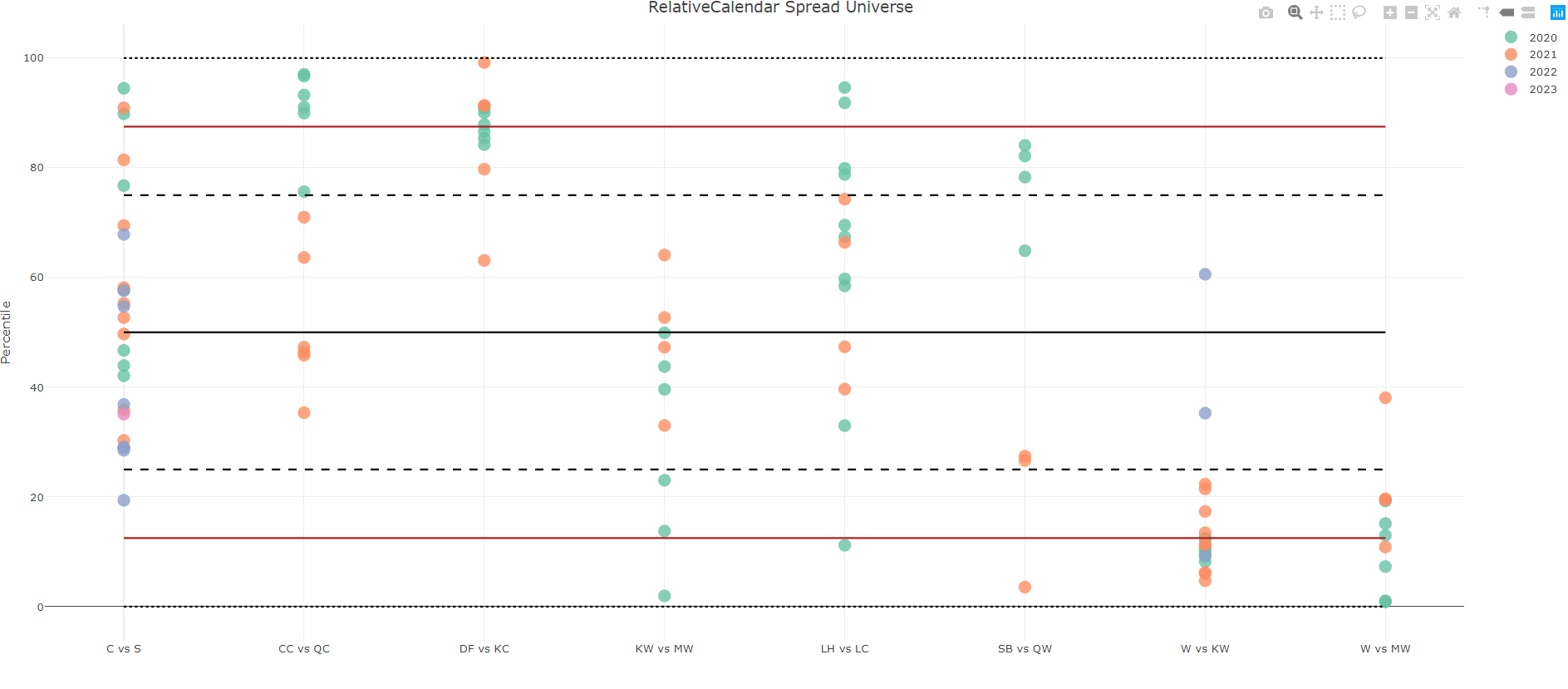
Other subtabs will be added over the next couple of weeks for some added functionality. Currently we have also added the scatterplot tab.
Remarks
In this post we introduce another way to express a a view on a relative values trade. A small subsample of our relative value universe is used for the beta testing. This will be extended witing the next couple of weeks.