Introduction
Some time ago we performed an events study on the Bridgeton Orders. In this write-up we tried to see if there were any short term signals we could possible extract from their daily data. The results were inconclusive but the interest in the data still remains. The data they generate basically amounts to reverse engineering trend following CTA signals to find prices where there might be significant buying and selling. A cautionary note is that trend following systems have notoriously low hit rates in and around the 40% mark, i.e. historically they are only correct four out of ten times. In this post we introduce the poor man’s Bridgeton Orders data which we dub Pseudo Bridgeton.
Basic Construction
For simplicity we define the trend signal to be the difference between the current price and a rolling mean price with some rolling window. For rolling windows we consider 10 to 258 trading days in steps of 2, giving 125 different rolling windows. If the signal is positive (negative) the system wants to enter a long (short) position. For each rolling window we determine the current signal together with the price move that will cause the signal to change, i.e. from long to short or the other way around. In this way we can get an idea of where systems with different lookbacks will change positions. We perform this calculation on two parts of the curve for each of the commodities we are interested in but other parts of the curve can easily be added.
Example Data
The table below shows an example of the output for March 2020 Corn. Consider the row with current signal NA and new signal zero. The price associated with this row coincides with the close of the previous day. All the rows above this reference row refer to trend systems that are currently short, here indicated by the -1 in current signal. Similalry the rows below the reference row indicate those systems which are currently long, here given by current signal equal to +1. The price column shows the value of the price where a collection number different trend systems will change their signal. As an example consider the top row. Here there are 12 systems that are currenlty short. If the C_H_2020 price drops to 411.47 by the close of today these systems will exit the short. Withing these 12 systems we find a minimum lookback of 156 and a maximum look back of 258 trading days. The collection of lookbacks average around 220 trading days. This corresponds to systems with long lookbacks and make out 9.52 percent of the different lookbacks considered.
| price | number | current signal | new signal | min lookback | max lookback | avg lookback | std lookback | fraction |
|---|---|---|---|---|---|---|---|---|
| 411.47 | 12 | -1 | 1 | 156 | 258 | 220.33 | 45.49 | 9.52 |
| 407.55 | 47 | -1 | 1 | 142 | 242 | 194.81 | 29.29 | 37.30 |
| 403.64 | 3 | -1 | 1 | 136 | 140 | 138.00 | 2.00 | 2.38 |
| 399.72 | 5 | -1 | 1 | 126 | 134 | 130.00 | 3.16 | 3.97 |
| 395.81 | 3 | -1 | 1 | 120 | 124 | 122.00 | 2.00 | 2.38 |
| 391.89 | 1 | -1 | 1 | 118 | 118 | 118.00 | NA | 0.79 |
| 391.50 | 1 | NA | 0 | 0 | 0 | 0.00 | NA | 0.00 |
| 387.19 | 20 | 1 | -1 | 10 | 116 | 71.20 | 32.05 | 15.87 |
| 383.28 | 25 | 1 | -1 | 16 | 106 | 66.88 | 31.24 | 19.84 |
| 379.36 | 9 | 1 | -1 | 26 | 42 | 34.00 | 5.48 | 7.14 |
If we suppose that the amount of capital used by all CTAs are equally distributed along the different lookback windows then we can use the table table to get an idea of the price levels were different CTAs will change their positioning.
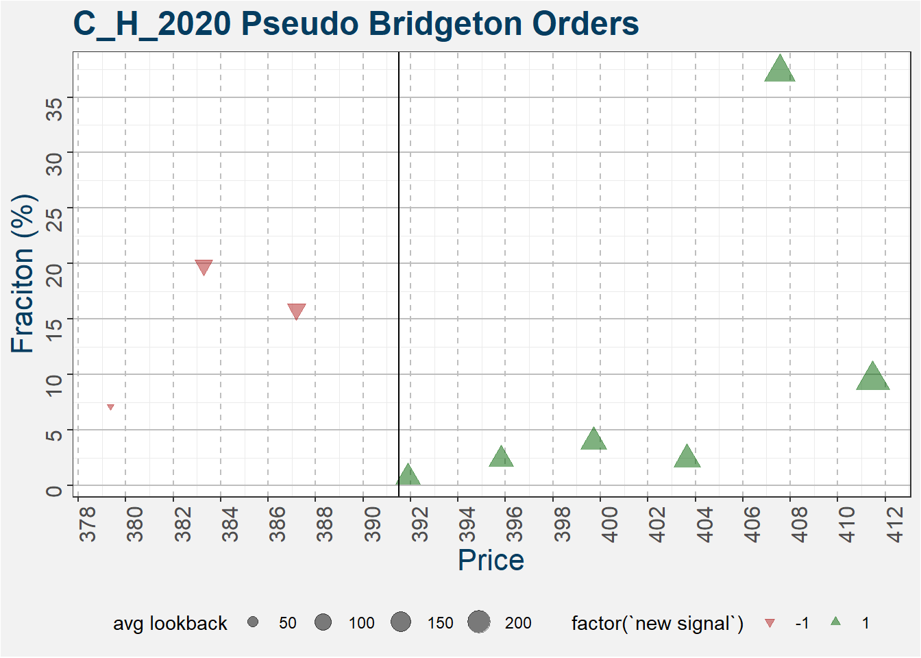
An interesting way to visualize the data is shown in the plot below. Here the vetical line represents the close of the previous day. Green triangles pointing upward indicate buy signals while red triangles pointing downward indicate sell signals. The size of the markers correspond to the fraction of lookback windows. Below we can see that the shorter lookback windows will get short at round 387 USd/bu and these make ap roughly 15% of the trend following CTAs. The longer dated systems are close to getting long March 2020 Corn, but in smaller increments, only at prices around 408 USd/bu do we start seeing substantial buying from the longer dated systems.

Remarks
This dataset has a couple crude assumptions that need to be taken with a pinch of salt. One of the biggest is the equal distribution of money among CTAs with short to long range trend following systems. The CTAs with the longest track records are those with longer windows, however they might not make up the bulk of the allocations.
As mentioned in the introduction we need to remind ourselves that trend following systems have low hit ratios. This means that most of the trades they put up are loosers. Their edge comes from positive skew which arises because of the way they manage their risk by cutting their losses and letting the winners run. This way the profitable trades pay for the loosers and hopefully add to the overall returns.