Introduction
When a simple question does not have a simple answer it might point to something interesting that is worth threading out. The simple question we attempt to solve deals with how to size up a relative value futures pairs trade so that it gives the best risk adjusted return. A couple examples we will consider include
- Ton for ton
- Equal notional exposure
- Equal volatility adjusted notional exposure
- Equal (at the money) implied volatility adjusted notional exposure
- Hedging ratio from cointegration test
- Machine Learning solution
We also explore the possible evolution of the hegding ratio as a function of fundamentals or seasonal input features, or even the shape of the futures curves of the underlying commodities.
For illustrative purposes we use the corn vs soybean (C vs S) spread for the remainder of the write-up. The table below gives the contract specifications of corn and soybeans. Notice that the tons per contract is basically equivalent, i.e. when sizing up the positions on a ton for ton basis we make use of a one to one ratio.
| comdty | units | constractsize | pricebasis | tonspercontract | multiplier |
|---|---|---|---|---|---|
| C | Long Bushels | 5000 | USd/Lbushel | 127.0072 | 50 |
| S | Short Bushels | 5000 | USd/Sbushel | 136.0791 | 50 |
We are interested in different parts of the futures curves of the inter commodity spread. We use the nomenclature tenor to denote the part of the curve we are interested in. Here, 0 refers to the front most part of the curve we are interested in. The greater the number the further along the curve the relative position will be entered. The table below shows the roll schedules of the different tenors. Notice that it can happend that the two commodities do not have the same contract code during a particular month and tenor. An example of this is January with tenor 4, here we are interested in the Z corn and F soybean contracts. In this particular case the Z corn contract will have expiry during December of the same year while the F soybean contract will have expiry the following year.
| C | S | C | S | C | S | C | S | C | S | |
|---|---|---|---|---|---|---|---|---|---|---|
| January | H | H | K | K | N | N | U | U | Z | X |
| February | K | K | N | N | U | U | Z | X | H | F |
| March | K | K | N | N | U | U | Z | X | H | F |
| April | N | N | U | U | Z | X | H | F | K | H |
| May | N | N | U | U | Z | X | H | F | K | H |
| June | U | U | Z | X | H | F | K | H | N | K |
| July | U | U | Z | X | H | F | K | H | N | K |
| August | Z | X | H | F | K | H | N | K | U | N |
| September | Z | X | H | F | K | H | N | K | U | N |
| October | Z | F | H | H | K | K | N | N | U | U |
| November | H | F | K | H | N | K | U | N | Z | U |
| December | H | H | K | K | N | N | U | U | Z | X |
We define the hedging ratio \(k\) with respect to the spread \(S^{\prime}\) as
\[ S^{\prime} = P_{S} - k P_{C} \]
where \(P_{S}\) and \(P_{C}\) denote the prices or notional values of S and C respectively. In the following we study the hedging ratios \(k\) that would have given the best historical risk adjusted returns from trading the spreads \(\S^{\prime}\) on the long side. To measure risk adjusted return we make use of the Sharpe ratio. Throughout we assume for every one long position in S a short position of \(k\) in C.
Long Term Behaviour
A classic way to trade the corn vs soybean spread is on a ton-for-ton basis. This amounts to a hedging ratio \(k = 1\). The plot below shows the evolution of $1 invested in the spread from 1978. The different colours represent the different tenors. It is clear that the tenors closer to the front end of the curve produce the best returns.
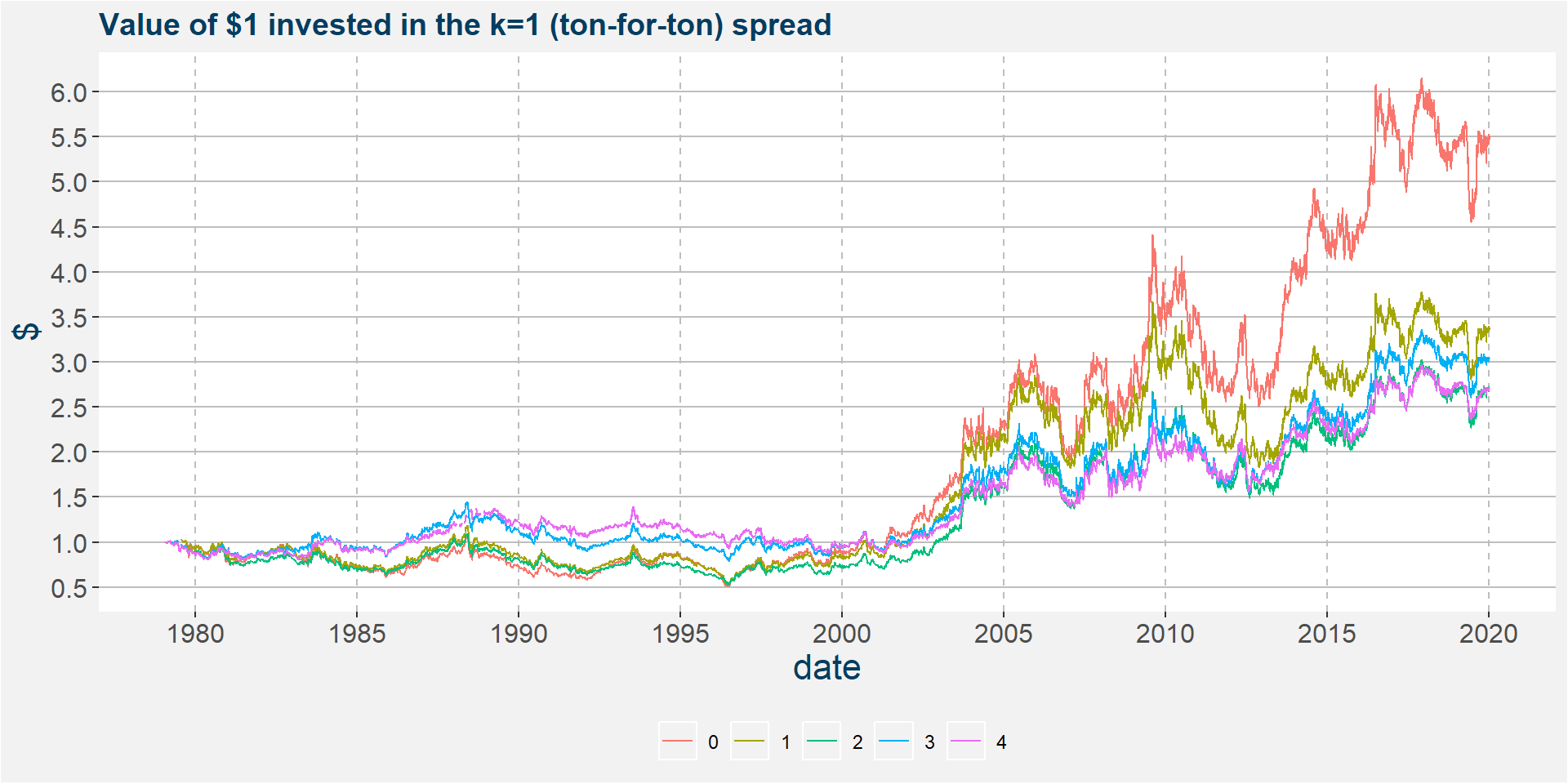
The table below summarises the return statistics of the corn vs soybean spread since 1978. Notice that the front end of the curve, tenor 0, gives the greatest annualised return and has the highest Sharpe ratio. Each column represents the different tenors we are interested in.
| 0 | 1 | 2 | 3 | 4 | |
|---|---|---|---|---|---|
| Annualized Return | 0.0432 | 0.0306 | 0.0249 | 0.0278 | 0.0250 |
| Annualized Std Dev | 0.1858 | 0.1743 | 0.1674 | 0.1611 | 0.1552 |
| Annualized Sharpe (Rf=0%) | 0.2324 | 0.1757 | 0.1489 | 0.1723 | 0.1613 |
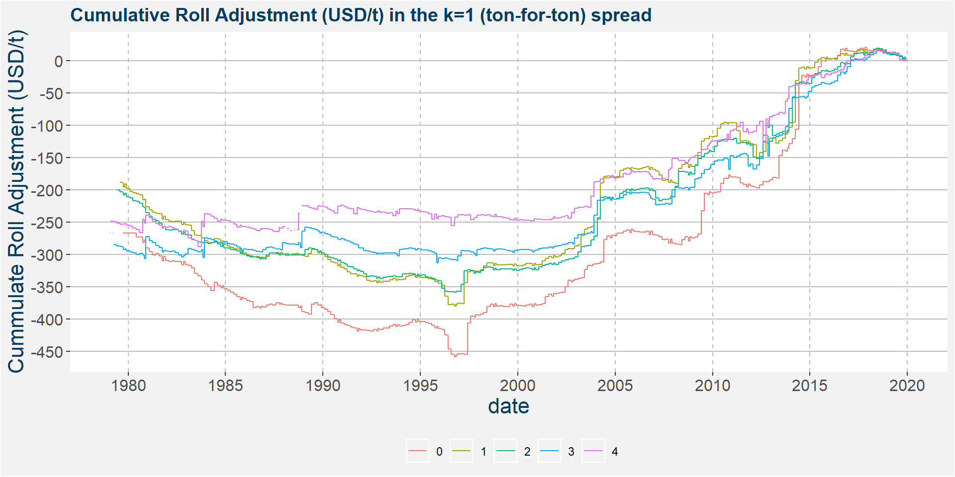
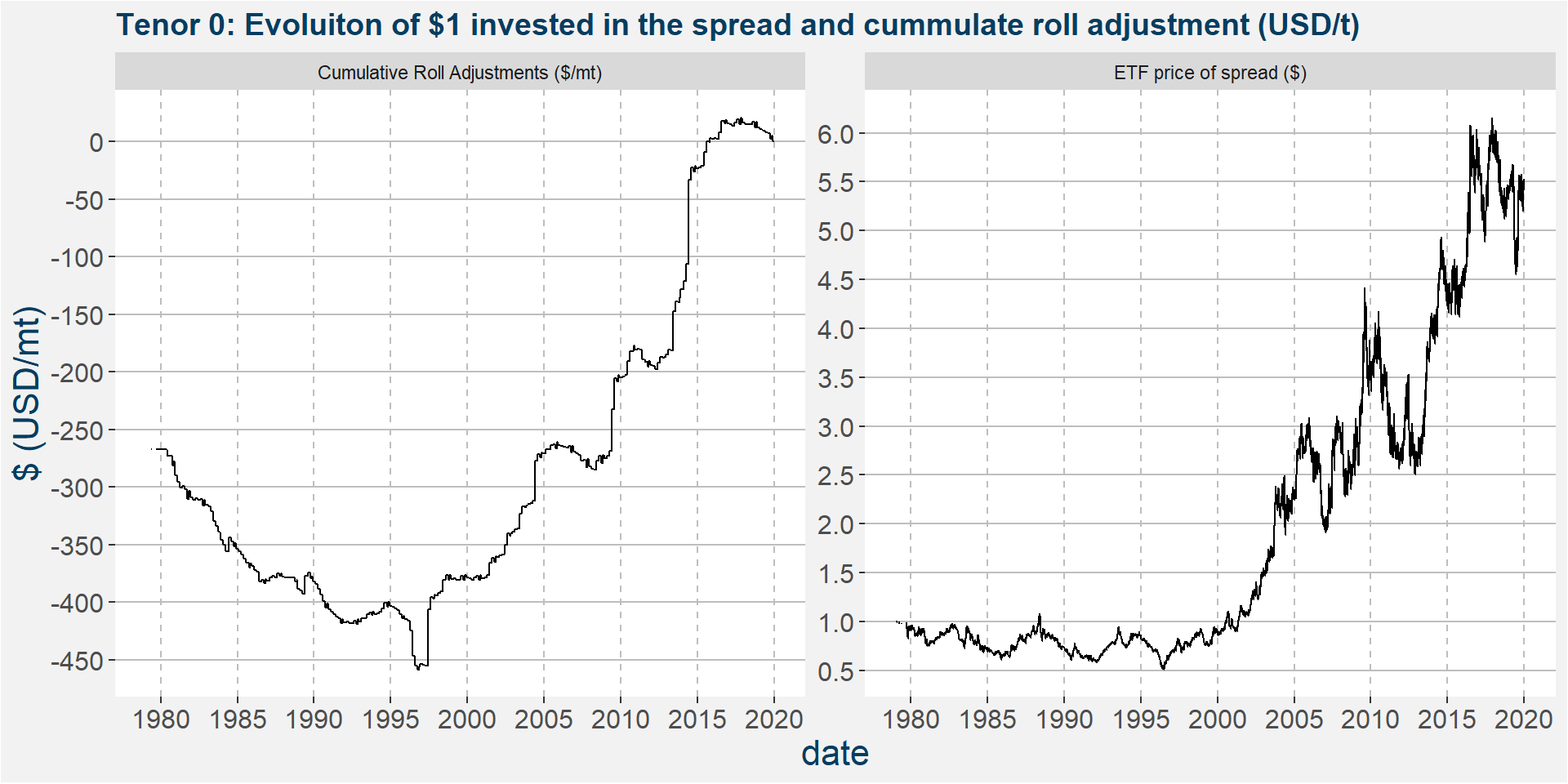
The plot below shows the cumulative roll adjustments in USD/t over the same period as the plot above. Notice that the slopes of the cumulative roll adjustments are negative prior to 2000 and positive thereafter. This implies that the roll return, by being long soybeans and short corn, was flat to negative prior to 2000. Conversely, the slopes are positive after 2000, showing a positive roll return on average. When we compare the above and below plots we can clearly see that the period of strong performance coincides with the period of positive roll returns. We will return to these ideas later.
Throughout we explore hedging ratios ranging from 0 to 5 with increments of 0.1. The plot below shows the Sharpe ratio of the corn vs soybean strategy as a function of the hedging ratio. The optimal Sharpe ratio is obtained when the slope of the graph is zero, ie. the turning point, indicated below by the dashed horizontal and vertical lines. Similar to before the different colours respresent the different tenors. The plots below were constructud using the full sample of data from 1978 to the most recent, hence the optimal hedging ratios are those for the entire duration of the sample.
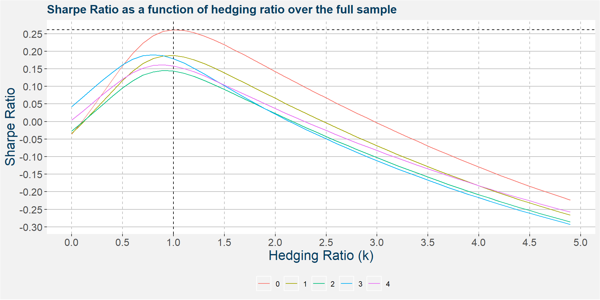
The table below shows the hedging ratios with the optimal Sharpe ratios for each of the tenors. Note that the full sample data gives the best risk adjusted reward with a hedging ratio of around 1. The table has columns denoted risk and reward. These amount to annualised standard deviation of returns and annualised return respectively.
| tenor | sharpe | risk | reward | hedging ratio |
|---|---|---|---|---|
| 0 | 0.2613302 | 18.56930 | 4.852719 | 1.0 |
| 1 | 0.1878358 | 17.40270 | 3.268851 | 1.0 |
| 2 | 0.1451596 | 15.87573 | 2.304514 | 0.9 |
| 3 | 0.1904283 | 14.71016 | 2.801231 | 0.8 |
| 4 | 0.1612735 | 14.71119 | 2.372525 | 0.9 |
The plot below show the Sharpe ratio as a function of hedging ratio split accross the time frames with predominantly negative and positive roll yields. These correspond roughly to dates before and after Jan 2000 respectively. From the plot below is is clear that the strategy performs much better under a positive roll yield with the risk ajusted returns between 4 and 5 time greater. It is interesting to note that the negative roll yield time frame showed the best risk adjusted return for a greater hedging ratio copared to the positive roll time frame. We will explore this later when we study the relationship between the cumulative roll adjustments and hedging ratio.
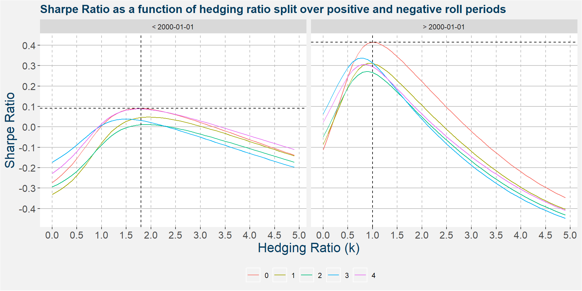
The table below shows the Sharpe and hedging ratios of the negative and positive roll yield time frames. Notice the large improvement in Sharpe ratio when the roll yields are positive. The lower hedging ratios associated with the period of prolonged positive roll might imply that the majority of the positive returns came from the long leg being in periods of sustained backwardation. If the optimal hedging ratio was larger it would imply that the short side was responsible for the majority of returns, i.e. being short in periods of prolonged contango.
| tenor | sharpe | hedging ratio | sharpe | hedging ratio |
|---|---|---|---|---|
| 0 | 0.0902240 | 1.8 | 0.4143883 | 1.0 |
| 1 | 0.0481139 | 2.0 | 0.3110130 | 0.9 |
| 2 | 0.0115402 | 1.9 | 0.2718790 | 0.9 |
| 3 | 0.0386196 | 1.5 | 0.3376391 | 0.8 |
| 4 | 0.0875275 | 1.8 | 0.3063408 | 0.8 |
Calendar Year Behaviour
Hedging Ratios
In this section we study the calendar year performance of the strategy, i.e. Jan-Dec behaviour. For each calendar year we determine the hedging ratio that yielded the highest Sharpe ratio. The results are shown in the plot below. Notice that thare are a couple of years where the optimal hedging ratio was zero, i.e. only a long position in soybeans was taken with no offsetting position in corn. Below we only show the results for tenor 0 since the other tenors’ results look similar.
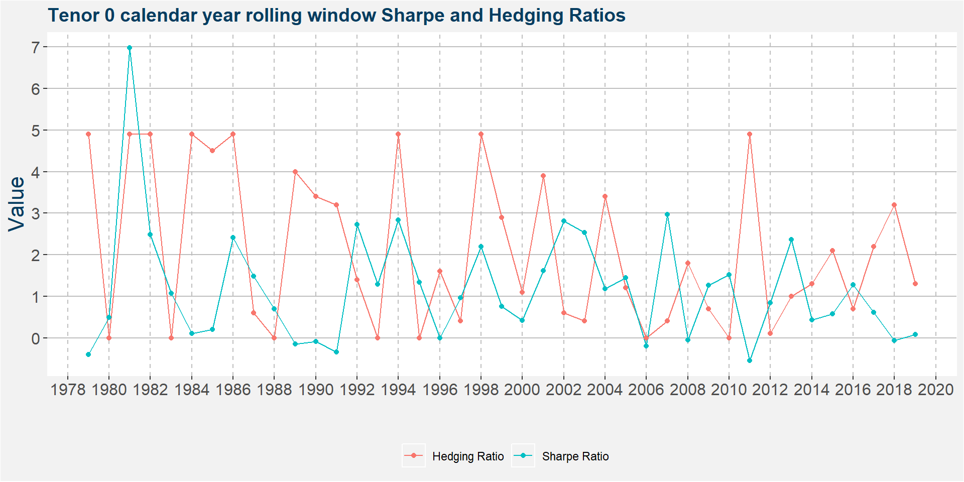
Notice that the majority of calendar years have positive Sharpe ratios. There are also many instances where the optimal hedging ratio was zero. We take a closer look at these cases below. The table below highlights those calendar years where the strategy had a negative Sharpe ratio. From the historical data we see that the 2011 calendar year had the worst performance.
| Hedging Ratio | Sharpe Ratio | tenor | year |
|---|---|---|---|
| 4.9 | -0.5456552 | 0 | 2011 |
| 4.9 | -0.4078986 | 0 | 1979 |
| 3.2 | -0.3416624 | 0 | 1991 |
| 0.0 | -0.1998812 | 0 | 2006 |
| 4.0 | -0.1503940 | 0 | 1989 |
| 3.4 | -0.0869361 | 0 | 1990 |
| 3.2 | -0.0638280 | 0 | 2018 |
| 1.8 | -0.0554524 | 0 | 2008 |
| 1.6 | -0.0056918 | 0 | 1996 |
The plot below shows the evolution of the tenor 0 spread (\(k=1\)) during 2011. Notice that the spread contracted by $2 during this period.
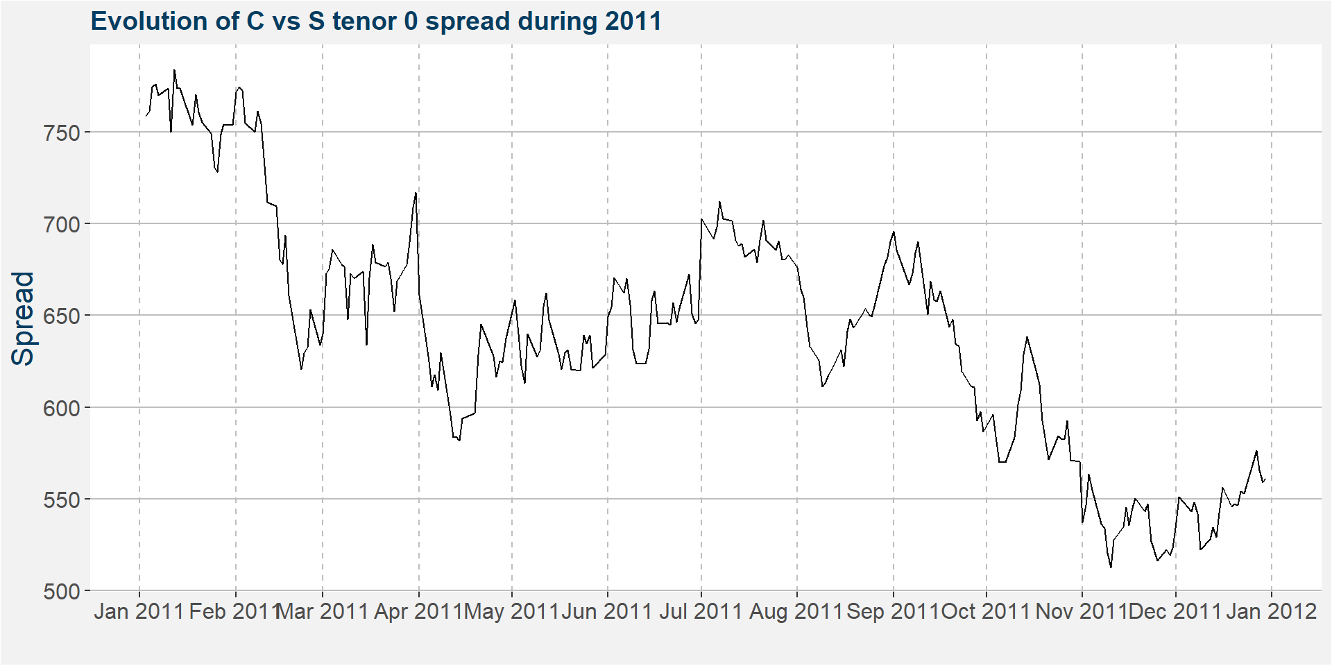
The collapse of the spread above can be attributed to a decrease in the price of soybeans. The plot below shows the value of $1 invested in the spread (\(k=1\)) on the first business day of 2011. Notice that corn rarely traded under a 5% loss while soybeans were down 30% during December 2011. It is also worthwhile to mention that these moves came off of high price ranges to begin with.
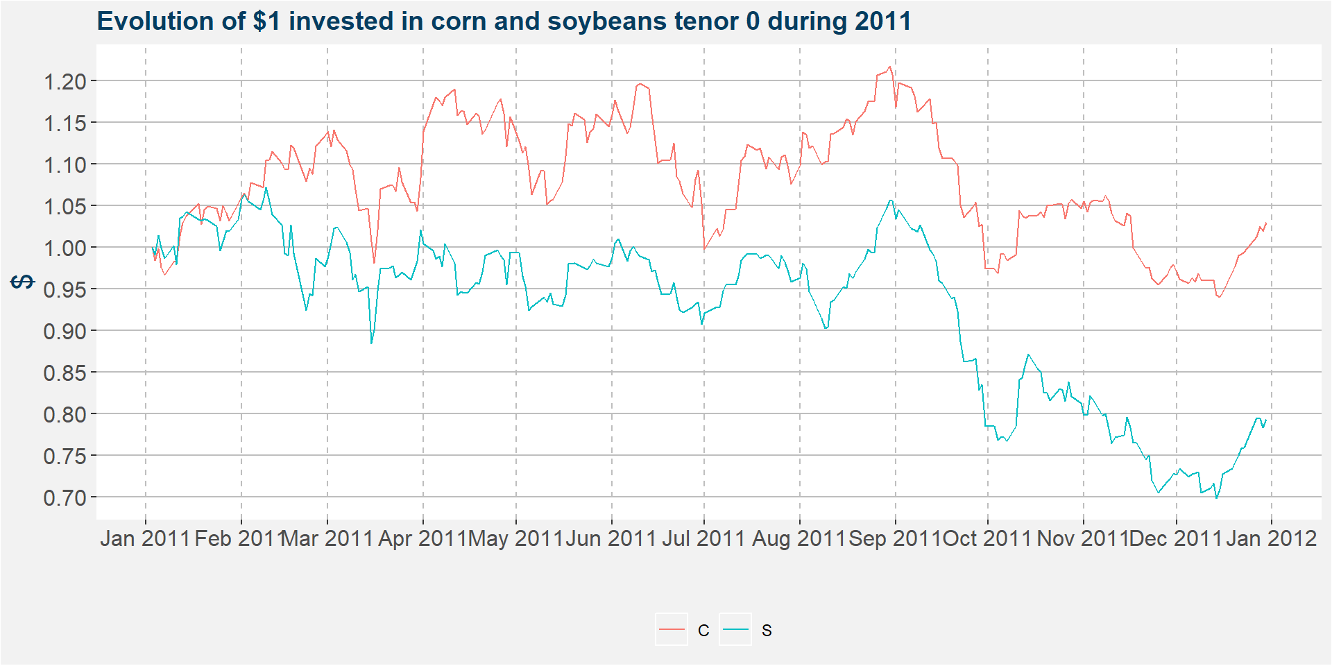
The only way that the hemorage could have been stopped, while being long the spread, would have been to increase the hedging ratio. The plot below shows the 2011 Sharpe ratio as a function of the hedging ratio. Notice that all the Sharpe ratios in the image are negative. The Sharpe ratio does become less negative with increasing hedging ratio.
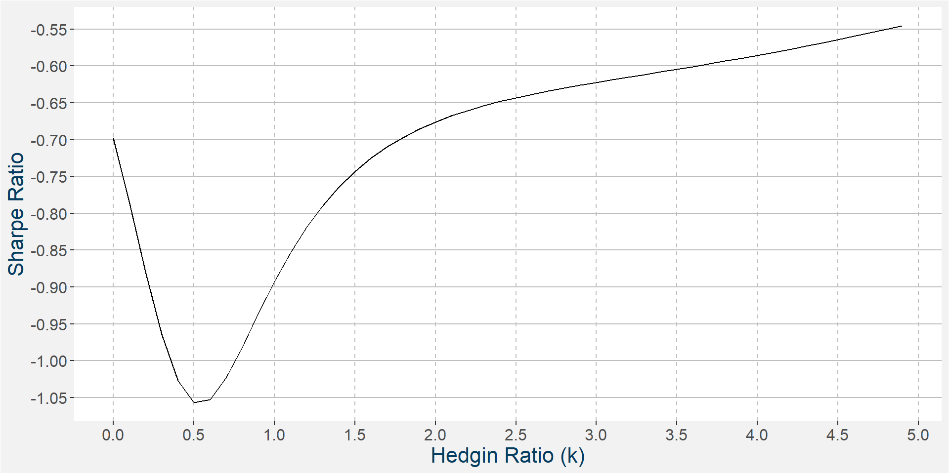
The table below hightights the results of the cases where the optimal hedging ratio was determined to be zero. Note these are the cases where it would have been best not to take a short corn position. A case that stands out, from a positive Sharpe ratio point of view, is the 2010 calendar year.
| Hedging Ratio | Sharpe Ratio | tenor | year |
|---|---|---|---|
| 0 | -0.1998812 | 0 | 2006 |
| 0 | 0.4896789 | 0 | 1980 |
| 0 | 0.6932677 | 0 | 1988 |
| 0 | 1.0689430 | 0 | 1983 |
| 0 | 1.2820173 | 0 | 1993 |
| 0 | 1.3378798 | 0 | 1995 |
| 0 | 1.5208971 | 0 | 2010 |
The plot below shows the value of $1 invested in the spread (\(k=1\)) during 2011. Notice that both corn and soybeans suffered some early losses of around 20%. By the end of the year soybeans was up 50% and corn was up 25%.
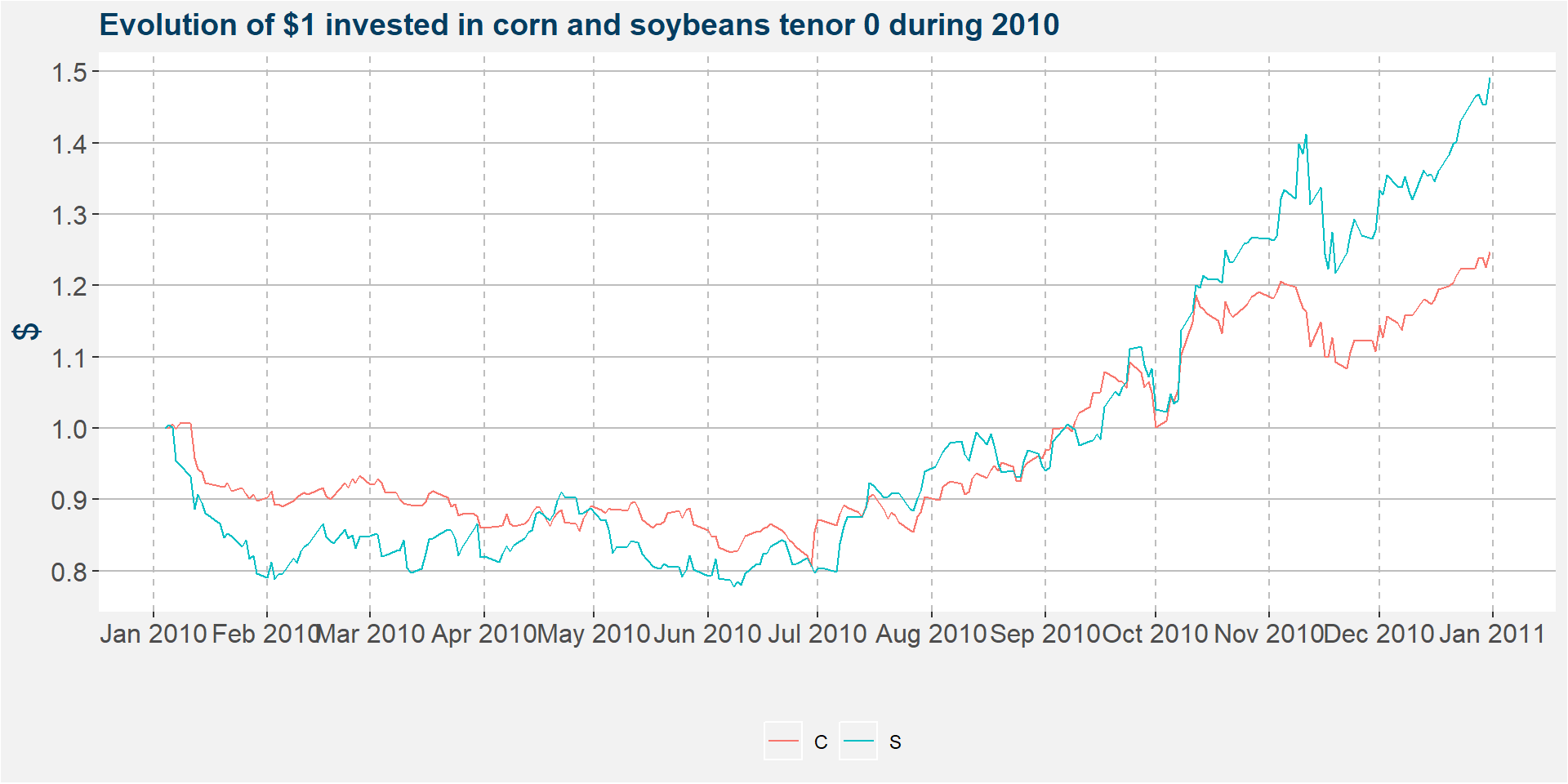
The performance statistics of beying long both of the commodities is given in the table below. Recall that the spread always takes up a long position in soybeans and a short corn. In this case it is clear that the return from the spread will have given the best results with a hedging ratio \(k=0\) since any short position in corn would have reduced the return from the spread.
| C | S | |
|---|---|---|
| Annualized Return | 0.3074 | 0.3435 |
| Annualized Std Dev | 0.3104 | 0.2179 |
| Annualized Sharpe (Rf=0%) | 0.9902 | 1.5762 |
Cumulative Roll Adjustments
A mathematical shorthand for the cumulative roll adjustment can be written as
\[ \text{CRA}_{S,C}(k) = \sum \Delta P_S - k \sum \Delta P_C \]
with
\[ \Delta P_S = P_S(\text{front}) - P_S(\text{deferred}) \] where \(\text{CRA}_{S,C}(k)\) denotes the cumulative roll adjustment with hedging ratio \(k\) between commodities S and C. \(P_S(\text{front})\) and \(P_S(\text{deferred})\) denotes the front and deferred parts of the curve, so that \(\Delta P_S\) is just the standard convention of a calendar spread. The cumulative roll adjustment of the spread can then be understood as the sum over all the calendar spreads of the two commodities over the respective roll periods taking the hedging ratio into account.
The plot below shows the cumulative roll adjustment and the value of $1 invested in the corn vs soybean spread since 1978. Notice that the cumulative roll gaps forms a long term envelope for the long term returns of the spread. The cumulative roll returns are calculated as the difference between the cumulative roll adjustments of the soybean and corn futures curves. This behaviour is seen for nearly all the fundementally linked pairs we consider, the interested reader is refered to this link for more examples. In the plots below we have set the hedging ratio to \(k=1\).
In the plot below we show the calenar year return as a funciton of cumulative roll adjustments. We highlight the zero percentage return line by the solid black line and superimpose a best fit linear regression to the data. Notice that the positive slope implies a larger cumulative roll adjustment coincides with a greater calendar year return. This can be stated differently as the greater the roll return the greater the overall return from the strategy. The roll return is determined by the curve shapes of the two underying commodities and is a point where we can enter the underlying fundamentals of the commodities making up the spread.
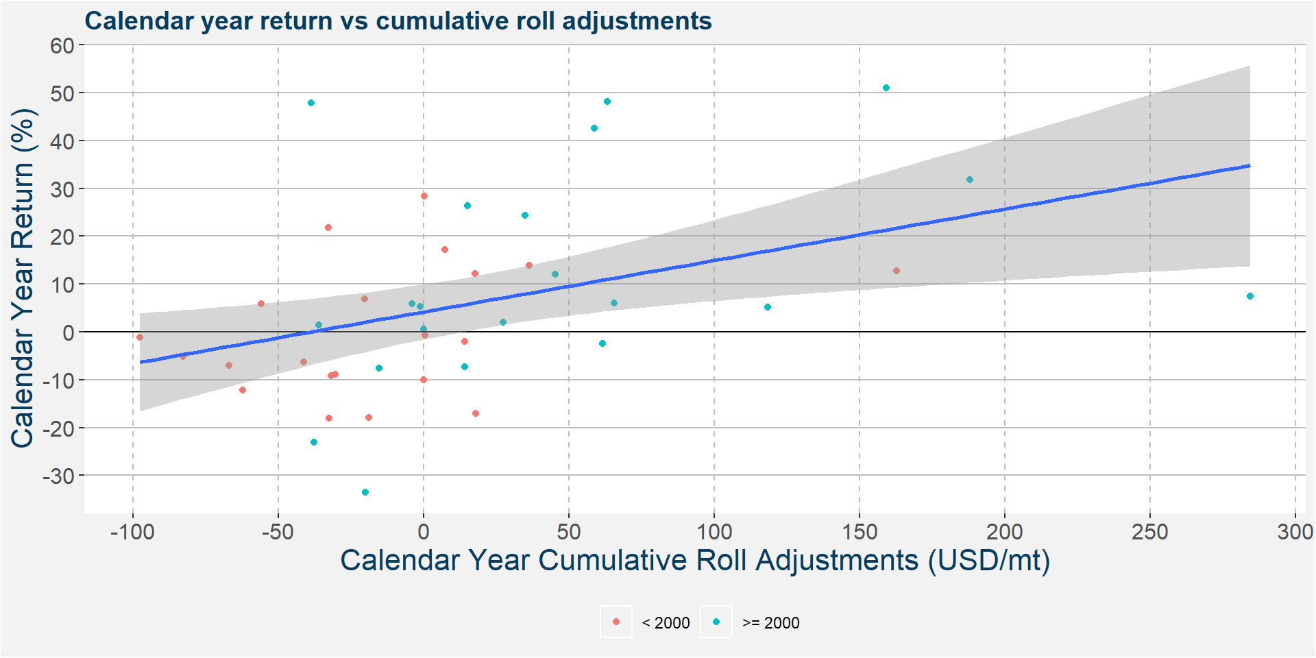
The table below summarises the calendar year results. The first column groups the calendar year returns with respect to their signs, +1 and -1 for positive and negative returns respectively. The bottom row shows the total for each of the columns. The values under the Cumulative Roll Adjustment heading show the number of calendar years with the specified sign of the return and cumulative roll adjustment. The first row shows that there was a total of 17 calendar years with negative returns. Of these 17 calendars years 12 showed a negative roll return. We can then ask, what is the probability of a negative roll return given a negative calendar year return, which we can calculate as
\[ P( \text{Negative Roll Return}| \text{Negative Calendar Year Return} ) = \frac{12}{17} \approx 70.6 \%. \]
Similarly we can consdier the column with positive Cumulative Roll Adjustment. We can see that there was a total of 22 calendar year with positive roll return. We can then ask, what is the probability of a positive calendar year return given a positive roll return, which we can calculate as
\[ P( \text{Positve Calendar Year Return}| \text{Positive Roll Return} ) = \frac{16}{23} \approx 69.6 \%. \]
| Return Sign | -1 | 1 | Total |
|---|---|---|---|
| -1 | 12 | 5 | 17 |
| 1 | 7 | 16 | 23 |
| Total | 19 | 21 | 40 |
If we are confident in achieving a positive roll return we can be reasonably sure that the calender year return will also be positive.
Rolling Time Frame Behaviour
In this section we consider the returns from 252 day rolling windows with seed days on WASDE report days in anticipation of down stream modelling with fundamental features as input parameters. Using this bootstrapping procedure we can determine some statistics on the hedging ratio over a large collection of yearly data that is not bound by the start and end of a calendar.
Hedging Ratio
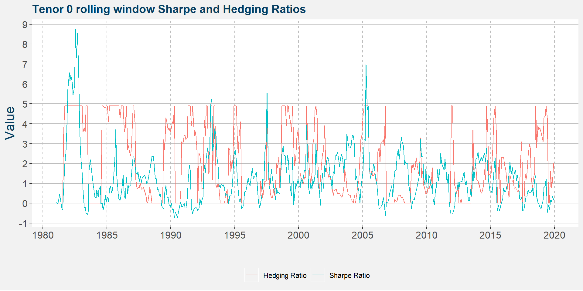
Similar to the calendar year case of the previous section we can see that negative Sharpe ratio’s seldom occur.
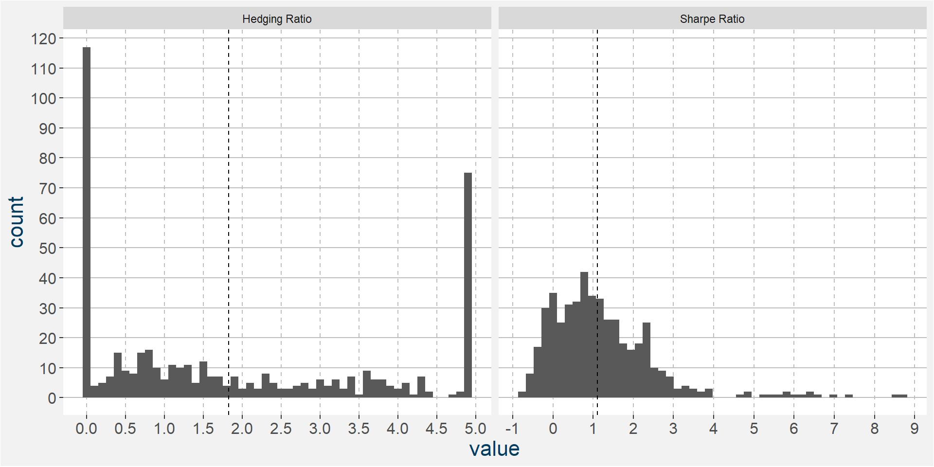
The plots below show the histograms of the hedging associated with the higherst Sharpe ratios respectively. Notice the clustering of heding ratios on the ends of the ranges. The left most cluster around \(k=0\) amounts to those cases where an outright long position in soybeans performed better than adding any short corn hedge. The cluster on the right hand side includes those occasions where holding a long position in soybeans proved to be detrimental and the hemorage can only be stopped by increasing the ratio of short corn to long soybeans. The dashed vertical lines represent the means of the datasets.
Cumulative Roll Adjustments
Similar to the calendar year case we see a positive slople when plotting the rolling yearly return as a function of the yearly cumulative roll adjustments. The colours of the dots represents seed dates before and after 2000-01-01 respectively.
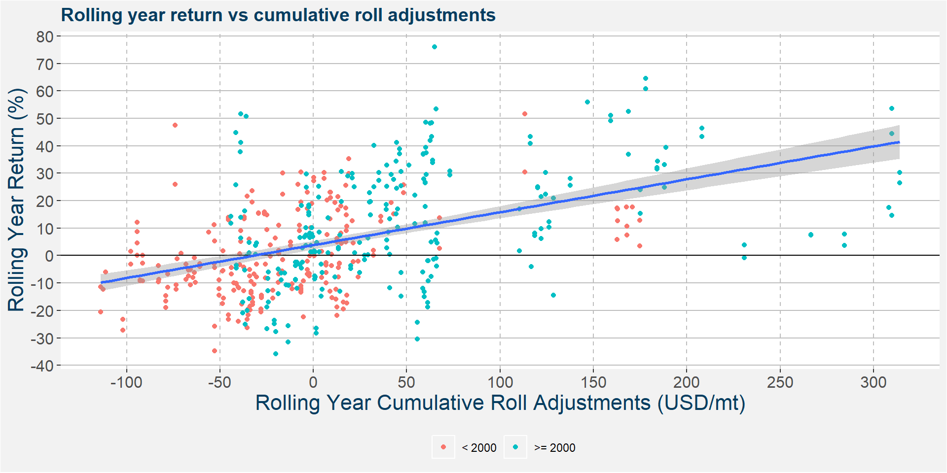
Similar to the calendar year case the table below shows the confusion matrix for the different sign of the yearly rolling returns and cumulative roll adjustments. In this case we get a whole lot more data and a better convergence of the probabilitites over a yearly rolling period.
| Return Sign | -1 | 1 | Total |
|---|---|---|---|
| -1 | 145 | 60 | 205 |
| 1 | 90 | 181 | 271 |
| Total | 235 | 241 | 476 |
Here too we can ask what is the probability of a positive yearly return given a positive roll return, which we can calculate as
\[ P( \text{Positve Yearly Return}| \text{Positive Roll Return} ) = \frac{181}{271} \approx 66.8 \%. \]
Hedging Ratio vs Cumulative Roll Adjustments
In this section we try to model the optimal hedging ratio as a functing of the cumulative roll adjustments on the rolling year basis, or at least to see if it might be possible.
The plot below shows the cumulative roll adjustments of corn and soybeans together with those of the spread with \(k=1\) as well as the \(k\)-corrected roll adjustments, these take the chosen \(k\) into account when calculating the cummulatie roll adjustments. The dashed red lines highlight the zero thresholds. For the corn and soybean cumulative roll adjustments the zero line signals the break between a majority contango (less than zero) and majority backwardated (greater than zero) curve.
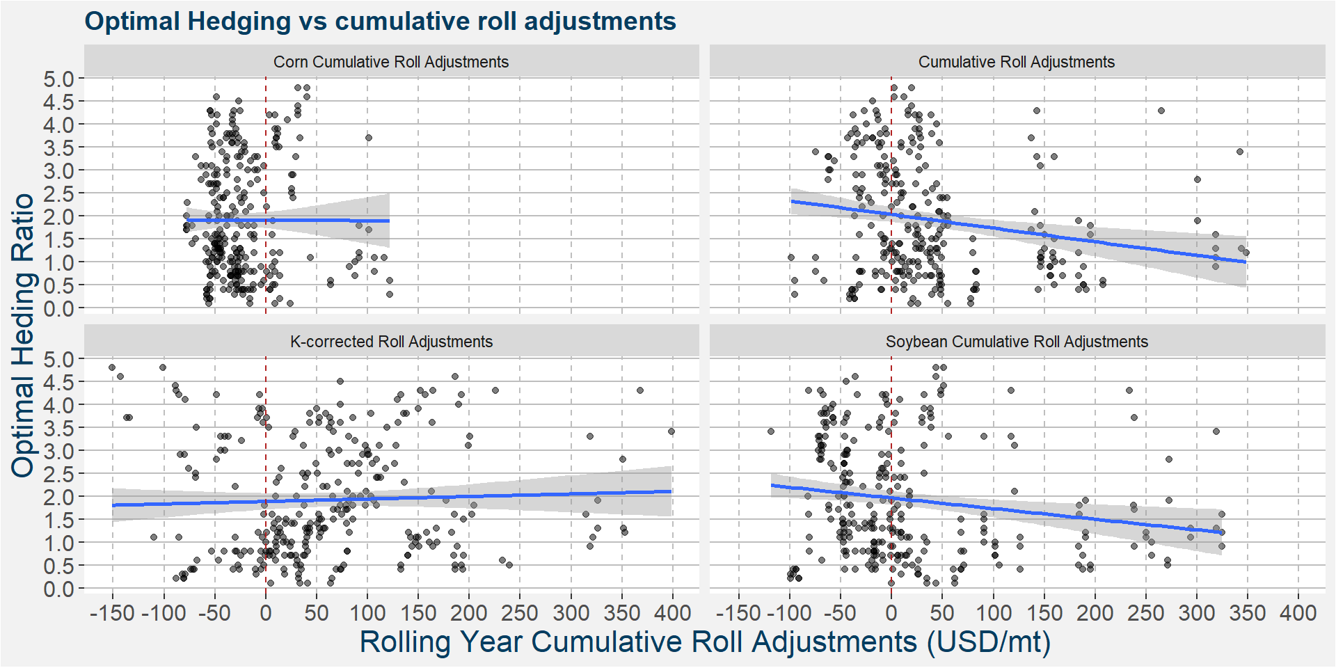
Naively we would have expected that, in the \(k=1\) case, the greater the cummulate roll adjustment the higher the hedging ratio shoud be. However, when we consider the top right facet we see a best fit linear curve with a negative slope, showing exactly the opposite conclusion. When correcting for the particular hedging ratios giving the optimal Sharpe ratios, bottom left facet, we see a slight upward sloping best linear fit. Notice also that in the \(k\)-corrected case the slope does not change substantially.
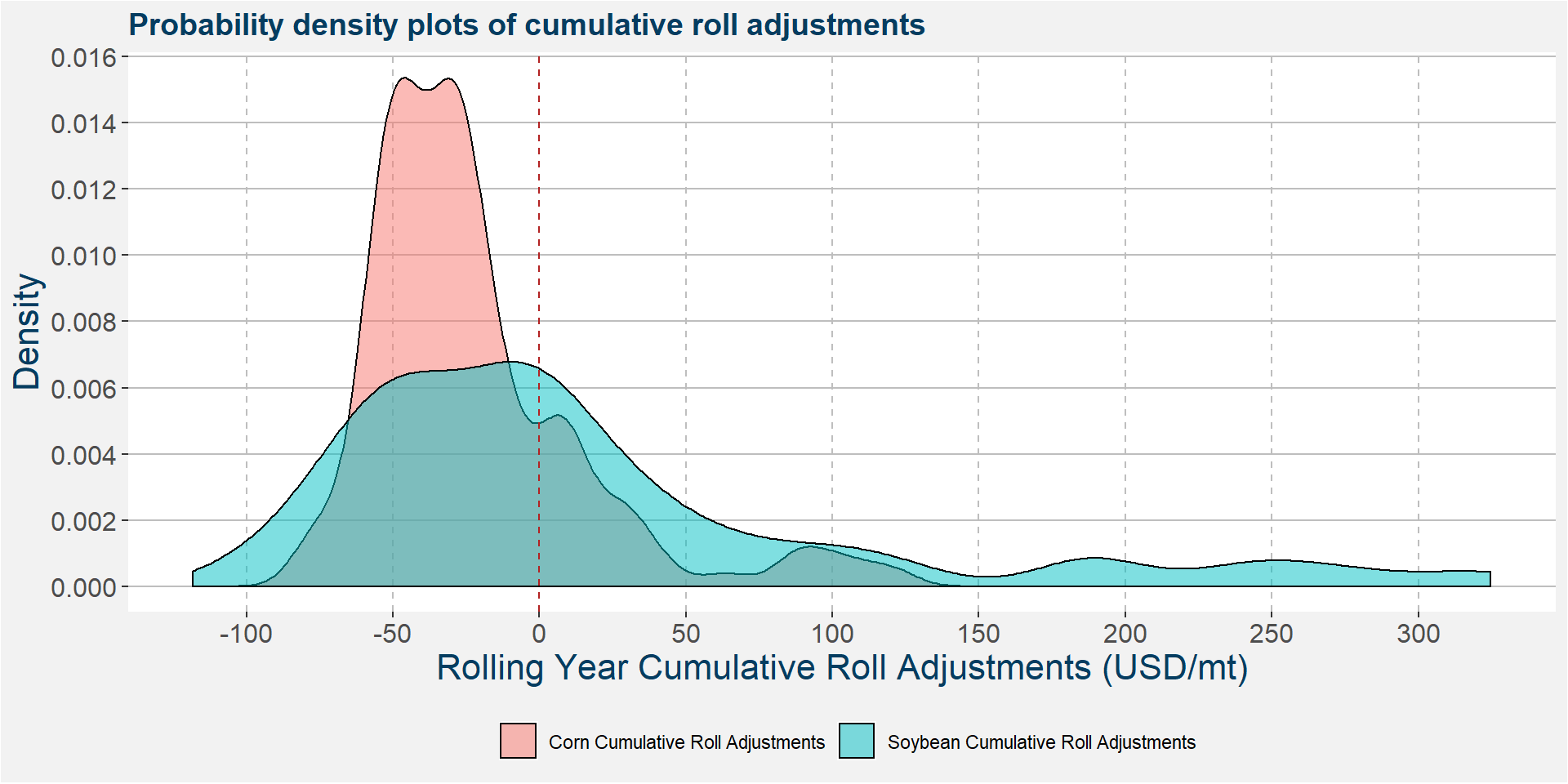
When we consider the cumulative roll adjustments of corn and soybeans on the same graph the differences in the roll behaviour becomes clear. From the image below we can see that corn predominantly trades in a contango and only rarely extends beyond the zero threshold. Contrast this with soybeans that have shown deep backwardation periods during rolls. If these deep backwardation periods are the ones responsible for the large cumulative roll adjustments of the spreads it would warrent a smaller hedging ratio \(k\) to gain the optimal Sharpe ratio.
Consider again the top right facet plot above showing the optimal hedging ratio as a function of rolling yearly cumulative roll adjustments for the spread with \(k=1\). There is an abrupt gap at a cumulative roll adjustment of 100 USD/mt. To the right of the 100 USD/mt line we see those cases with large roll returns. These high roll regimes occur over prolonged periods, we split each of the contiguous regions into a separete table below.
The table below shows the time period from 1997-06-12 to 1998-05-12. Early on we see the corn spread being backwardated before slipping into contango. The soybean curve remained agressively backwardated during this period. The table underneath the time frame data gives the statistics of the Sharpe and hedging ratios accross the time frame.
| Date | Sharpe | Hedging | C Roll Adjusts | S Roll Adjusts | Roll Adjusts | k-corrected |
|---|---|---|---|---|---|---|
| 1997-06-12 | 3.11 | 1.1 | 43.75 | 190.75 | 147.00 | 142.62 |
| 1997-07-11 | 5.42 | 4.9 | 43.75 | 190.75 | 147.00 | -23.63 |
| 1997-08-12 | 2.19 | 1.9 | 7.00 | 190.75 | 183.75 | 177.45 |
| 1997-09-12 | 0.89 | 1.2 | 7.00 | 190.75 | 183.75 | 182.35 |
| 1997-10-10 | 1.20 | 0.5 | 7.00 | 195.50 | 188.50 | 192.00 |
| 1997-11-10 | 1.92 | 0.4 | 4.00 | 195.50 | 191.50 | 193.90 |
| 1997-12-11 | 1.41 | 0.4 | 4.00 | 187.50 | 183.50 | 185.90 |
| 1998-01-13 | 0.96 | 0.7 | 4.00 | 187.50 | 183.50 | 184.70 |
| 1998-02-11 | 0.90 | 0.5 | -4.75 | 184.00 | 188.75 | 186.38 |
| 1998-03-12 | 0.35 | 0.9 | -4.75 | 184.00 | 188.75 | 188.28 |
| 1998-04-09 | 0.89 | 1.8 | -11.25 | 184.25 | 195.50 | 204.50 |
| 1998-05-12 | 0.63 | 1.6 | -11.25 | 184.25 | 195.50 | 202.25 |
| variable | Average | Stdev | p25 | Median | p75 |
|---|---|---|---|---|---|
| Sharpe | 1.655833 | 1.410767 | 0.89 | 1.08 | 1.9875 |
| Hedging | 1.325000 | 1.247634 | 0.50 | 1.00 | 1.6500 |
The table below represents the period from 2004-06-10 to 2005-04-08. Here we see strong contango periods in corn coupled with strong backwardation in soybeans. Notice the high hedging ratio which implies the greatest risk adjusted return was achieved with a greater short position in corn.
| Date | Sharpe | Hedging | C Roll Adjusts | S Roll Adjusts | Roll Adjusts | k-corrected |
|---|---|---|---|---|---|---|
| 2004-06-10 | 1.24 | 0.0 | -17.75 | 126.00 | 143.75 | 126.00 |
| 2004-07-12 | 1.53 | 0.4 | -17.75 | 126.00 | 143.75 | 133.10 |
| 2004-08-12 | 0.99 | 0.9 | -20.00 | 126.00 | 146.00 | 144.00 |
| 2004-09-10 | 0.76 | 1.1 | -20.00 | 126.00 | 146.00 | 148.00 |
| 2004-10-12 | 0.11 | 2.1 | -20.00 | 120.75 | 140.75 | 162.75 |
| 2004-11-12 | 0.78 | 3.1 | -25.25 | 120.75 | 146.00 | 199.03 |
| 2004-12-10 | 1.19 | 3.3 | -25.25 | 117.25 | 142.50 | 200.57 |
| 2005-01-12 | 1.69 | 4.3 | -25.25 | 117.25 | 142.50 | 225.82 |
| 2005-02-09 | 3.34 | 4.9 | -27.50 | 122.75 | 150.25 | 257.50 |
| 2005-03-10 | 3.26 | 4.9 | -27.50 | 122.75 | 150.25 | 257.50 |
| 2005-04-08 | 7.19 | 4.9 | -30.00 | 114.25 | 144.25 | 261.25 |
| variable | Average | Stdev | p25 | Median | p75 |
|---|---|---|---|---|---|
| Sharpe | 2.007273 | 1.987149 | 0.885 | 1.24 | 2.475 |
| Hedging | 2.718182 | 1.906210 | 1.000 | 3.10 | 4.600 |
Next we consider the period from 2009-06-10 to 2010-04-09. Here we see very strong contango curves in corn couples with strong backwardated curves in the soybean market.
| Date | Sharpe | Hedging | C Roll Adjusts | S Roll Adjusts | Roll Adjusts | k-corrected |
|---|---|---|---|---|---|---|
| 2009-06-10 | 1.47 | 1.5 | -69.0 | 91.00 | 160.00 | 194.50 |
| 2009-07-10 | 3.17 | 3.3 | -69.0 | 91.00 | 160.00 | 318.70 |
| 2009-08-12 | 2.19 | 1.3 | -59.0 | 91.00 | 150.00 | 167.70 |
| 2009-09-11 | 2.23 | 1.6 | -59.0 | 91.00 | 150.00 | 185.40 |
| 2009-10-09 | 1.16 | 1.0 | -59.0 | 101.75 | 160.75 | 160.75 |
| 2009-11-10 | 0.79 | 0.7 | -54.5 | 101.75 | 156.25 | 139.90 |
| 2009-12-10 | 1.55 | 0.5 | -54.5 | 105.50 | 160.00 | 132.75 |
| 2010-01-12 | 0.70 | 0.5 | -54.5 | 105.50 | 160.00 | 132.75 |
| 2010-02-09 | 0.66 | 0.9 | -54.5 | 101.50 | 156.00 | 150.55 |
| 2010-03-10 | 1.28 | 0.7 | -54.5 | 101.50 | 156.00 | 139.65 |
| 2010-04-09 | 1.08 | 1.0 | -56.0 | 91.00 | 147.00 | 147.00 |
| variable | Average | Stdev | p25 | Median | p75 |
|---|---|---|---|---|---|
| Sharpe | 1.480000 | 0.7737571 | 0.935 | 1.28 | 1.87 |
| Hedging | 1.181818 | 0.7947555 | 0.700 | 1.00 | 1.40 |
Finally we consider the period from 2013-06-12 to 2015-04-09 where the effects of the drought caused both the corn and soybean curves to be in prolonged periods of backwardation. After the drought the corn curve corrected back to a contango much fasther than that of soybeans.
| Date | Sharpe | Hedging | C Roll Adjusts | S Roll Adjusts | Roll Adjusts | k-corrected |
|---|---|---|---|---|---|---|
| 2013-06-12 | 0.78 | 0.0 | 82.50 | 238.25 | 155.75 | 238.25 |
| 2013-07-11 | 0.37 | 0.9 | 82.50 | 238.25 | 155.75 | 164.00 |
| 2013-08-12 | 1.85 | 3.7 | 101.25 | 238.25 | 137.00 | -136.38 |
| 2013-09-12 | 1.12 | 1.7 | 101.25 | 238.25 | 137.00 | 66.12 |
| 2013-11-08 | 2.21 | 1.8 | 91.50 | 237.75 | 146.25 | 73.05 |
| 2013-12-10 | 2.31 | 1.2 | 91.50 | 250.25 | 158.75 | 140.45 |
| 2014-01-10 | 2.58 | 1.1 | 91.50 | 250.25 | 158.75 | 149.60 |
| 2014-02-10 | 2.04 | 1.0 | 87.50 | 255.75 | 168.25 | 168.25 |
| 2014-03-10 | 2.13 | 0.7 | 87.50 | 255.75 | 168.25 | 194.50 |
| 2014-04-09 | 2.30 | 0.5 | 63.50 | 271.00 | 207.50 | 239.25 |
| 2014-05-09 | 2.16 | 0.6 | 63.50 | 271.00 | 207.50 | 232.90 |
| 2014-06-11 | 2.40 | 0.9 | 6.50 | 324.75 | 318.25 | 318.90 |
| 2014-07-11 | 2.61 | 1.6 | 6.50 | 324.75 | 318.25 | 314.35 |
| 2014-08-12 | 2.24 | 1.2 | -23.50 | 324.75 | 348.25 | 352.95 |
| 2014-09-11 | 2.86 | 4.9 | -23.50 | 324.75 | 348.25 | 439.90 |
| 2014-10-10 | 1.71 | 3.4 | -23.50 | 319.00 | 342.50 | 398.90 |
| 2014-11-10 | 1.19 | 1.3 | -25.00 | 319.00 | 344.00 | 351.50 |
| 2014-12-10 | 0.76 | 1.3 | -25.00 | 293.75 | 318.75 | 326.25 |
| 2015-01-12 | 0.81 | 1.1 | -25.00 | 293.75 | 318.75 | 321.25 |
| 2015-02-10 | 0.60 | 1.9 | -28.00 | 272.75 | 300.75 | 325.95 |
| 2015-03-10 | 1.07 | 2.8 | -28.00 | 272.75 | 300.75 | 351.15 |
| 2015-04-09 | 1.64 | 4.3 | -31.25 | 233.75 | 265.00 | 368.12 |
| variable | Average | Stdev | p25 | Median | p75 |
|---|---|---|---|---|---|
| Sharpe | 1.715455 | 0.7479924 | 1.0825 | 1.945 | 2.285 |
| Hedging | 1.722727 | 1.2909693 | 0.9250 | 1.250 | 1.875 |
What we have learned so far
- Over the entire historical sample a hedging ratio of 1 gives the best risk adjusted return
- Much greater risk adjusted returns can be achieved during periods of positive cumulative roll
- If we are certain of a positive cummmulative roll there is a high (70%) probability of a positive return
- Historical large cumulative roll adjustments were due to sustained periods of backwardation in soybeans which are sometimes coupled with a corn curve moving toward a stronger contango
- In cases where corn is forecasted to be the driving factor of the spread and rolls a greater hedging ratio needs to be taken compared to when soybeans will be the driving factor.
- The above implies that during weather stress periods it is good practice to have a lower hedging ratio