1 Introduction
In this document, we give some detail about the relative value commodity universe in which the Polar Star Limited fund invests. We start by assuming the reader has zero experience with the futures market and derivative instruments. We do however assume some familiarity with financial markets in general.
2 Nomenclature
In the commodity and futures space, there are some unique words and phrases that a reader form an equity background might not be familiar with. If the reader is familiar with commodity trading this section can be skipped. Where necessary links to the definitions will be included in the text following this section. Below we give a list of commonly used words with some definitions:
Spread
Traders refer to the spread as the price difference between two different assets. Throughout, when we write the spread of A vs B we define the spread \(S\) as \[ S = P_{B} - P_{A} \] where \(P_{i}\) if the price of asset \(i\).
Curve or Term Structure
Unlike a share in a company, futures contracts expire. If you are long (short) a futures contract at expiry you need to take (make) delivery of the underlying asset. Different expiries have different prices. When the different prices are shown graphically as a function of expiry dates we refer to this as the curve or futures curve. Readers with a background in fixed income should be familiar with this notion. Similarly, those readers that hedge out currency exposure will be familiar with the forward curve. In essence, the curve is the same idea.
Contango
When futures contracts with a further dated expiry is priced at a premium compared to nearer dated expiries we say the curve is in contango. We might also say the spread \[ S = P_{\text{near dated}} - P_{\text{far dated}} \] is negative.
Backwardation
When futures contracts with a further dated expiry is priced at a discount compared to nearer dated expiries we say the curve is in backwardation. We might also say the spread \[ S = P_{\text{near dated}} - P_{\text{far dated}} \] is positive.
-
Suppose we hold a long (short) position in a futures contract. When expiry approaches and we want to keep our long (short) exposure, without taking (making) delivery, we need sell (buy) our current position and buy (sell) the futures contract with the next available, or later, expiry. This process is called rolling forward. When the act of rolling yields a profit (loss) we call it a positive (negative) roll.
Calendar Spread
Any trade where we take opposing positions on the futures curve of the same commodity. There are two types of calendar spreads, Bull and Bear Spreads. Bull (Bear) spreads take long (short) exposure on the near-dated and short (long) exposure on the far-dated parts of the futures curve.
Inter-Commodity Spread
Any trade where we take opposing positions on the futures curve of two, or more, commodities.
-
When doing long time-frame statistics on the prices of futures contracts we need to take the roll and the shape of the curve into account. During each roll, we have to shift the entirety of the historical price data upward (downward) in the case of a contango (backwardated) roll. We make use of a linear price shift equal to the difference in price between the near and far-dated futures contract. We refer to this number is the gap. The historical shift amounts to the cumulative gap.
3 Curve Shape
3.1 Backwardation and Contango
In this section, we show an example of curve structures in contango and backwardation. Backwardation and contango refer to the shape of a futures curve. A curve is in backwardation when further dated futures contracts are priced at a discount compared to the near-dated or front contract. Contango is exactly the opposite and refers to the state where the further-dated part of the curve is priced at a premium compared to the front month.
Below we show an example of a futures curve in contango, in this case, the corn curve as seen on 2019-06-12.
Let us now make the simplifying assumption that the front month price or spot market price of corn remains fixed at the current levels, here shown to be 430. If we have long exposure in corn and want to keep that long exposure, we need to sell the front month and buy the following contract. This process is called rolling. In the example above it implies you have to buy the C U9 Comdty contract for 438.25. This price will now decrease toward the spot market as it matures toward expiry, leaving you with a loss of -8.25 cents per bushel. This is an example of a negative roll. Hence, if you want to profit from long exposure in a commodity with a curve that is in contango you need to clear the barrier set by rolling your position along the futures curve.Below we show an example of a curve in backwardation.
It is much easier to trade long exposure profitably in a commodity that is in backwardation. Similar to the case of corn we suppose the spot price for zinc is fixed at the current levels of 2617.5. When the front contract expires and we want to keep our long exposure, we have to sell the front month at 2617.5 and buy the next contract at 2559.5. Assuming the shape of the curve remains constant this gives you a profit of 58 USD/MT. This is an example of a positive roll.
3.2 The driver of long-term returns
Literature is abundant on the long-term driver of commodity returns. The largest of these drivers is the term structure or curve shape of the commodity. Below we list a couple of academic papers by Hilary Till on the subject of the terms structure as the main driver of commodity futures returns:
- Term Structure as the Primary Driver of Long-Term Commodity Futures Returns
- Long-Term Sources of Return in the Commodity Futures Markets: Evidence from the Grain Markets
- A Long-Term Perspective on Commodity Futures Returns
Another classic article is The Strategic and Tactical Value of Commodity Futures by Erb and Harvey. This one is a must-read for all commodity investors.
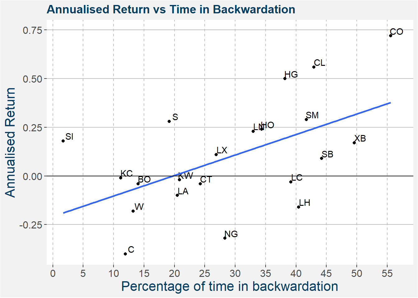
Inspired by the work of Till we created the image below. We show the annualised return for a collection of commodities in a long-only allocaiton as a function of time spent in backwardation. The superimposed curve shows the best fit linear regression. From the image below it is clear that the more time a commodity spends in backwardation the greater its returns from a long-only point of view.
4 Relative Value commodity Universe
We consider two types of relative value exposures in the global commodities markets,
- Calendar Spreads and
- Inter-Commodity Spreads.
We have two broad methods of identifying trade opportunities. The first is from a quantitative basis where we look at each of the spreads that are either stretched or suppressed when compared to historical values. These define a reduced collection of possible convergence trades where we would like to earn a profit from the spreads returning to a more normal range. The fundamentals associated with the commodities inside the reduced collection is then studied. The aim is to find a fundamental reason why a particular spread is stretched or suppressed. If the fundamentals do not support the value of the spread we include the trade on a shortlist of opportunities to consider for further investigation.
The image below gives an example of what the Relative Spread or Inter-Commodity Spread universe looks like. The y-axis shows the percentile of the current spread compared to historical values. The x-axis shows the different inter-commodity spreads we are interested in. Each dot represents a possible trade, i.e. the spread between two futures contracts of different commodities. We consider spreads to be suppressed (stretched) is they are below (above) the bottom (top) red line. In this way, we consider trades from the outside in.

The second approach enters from the point of view of global fundamentals. Fundamentals in the case of commodity markets are comprised of the balance sheets of the largest producing and consuming nations. Given the current weather, political scenario, freight rates, and historical values we forecast the fundamentals of the main players in each of the commodity markets. Given these forecasts, we determine the likely values of the spreads. If the possible return from the spread and the roll give a positive result we add this on a shortlist of opportunities. These type of trades form a collection of possible divergence trades.
Suppose we have obtained our shortlist of opportunities that we would like to investigate further. The next part is to determine the risk associated with each of the listed opportunities. We do not think of risk as the standard deviation of daily returns, as is the practice in the industry. Rather, we think of risk as being associated with the uncertainty in the underlying fundamentals of the different commodity markets. Consequently, we stress the underlying fundamentals in such a way that the subsequent price moves will be opposite to the direction of the trade we are interested in taking. As an example, for the grains markets, we will consider years with droughts or other adverse weather scenarios and the effect that had on the global balance sheets, and spread and roll behaviour. As a rule of thumb, defining risk this way, we only consider trades with an asymmetric two-to-one return to risk profiles.
When it comes to sizing a trade we use a 1% of NAV risk rule of thumb. Stated differently, if the stressed scenario occurs and the spreads moves against us, we are prepared to lose 1% of our assets. However, if the underlying fundamentals have not changed we will hold on to the position and will not be stopped out. In the case of a stressed spread, it will be even more stressed without fundamental support and would remain a sound trade according to our methodology. On the other hand, if the fundamentals have changed in such a way that the trade is not supported we will trade out of the position.
Below we delve deeper into each of these opportunities and give some examples.
4.1 Calendar Spreads
A calendar spread is a relative value trade between different parts of the futures curve of the same commodity. Taking a view on a calendar spread is akin to taking a view on the term structure of the commodity.
Four main factors are contributing to the shape of a commodity futures curve
- Funding and storage costs,
- Expected supply and demand imbalances,
- Convenience yields and
- Hedging pressure.
The cost of storing a commodity for later delivery forces the far dated parts of the futures curve upward, i.e. more contango. A decline in storage costs should coincide with a decrease (increase) in the degree of contango (backwardation) of a commodity. There have been, and continue to be, varying storage costs in the United States Wheat market that have affected the curve shapes. Additionally, there is an opportunity cost associated with the storage of a commodity. The funding used in the storing process could have been invested in a risk-free government bond. For this reason, a higher (lower) interest rate corresponds to a greater (smaller) degree of contango to compensate for the opportunity cost.
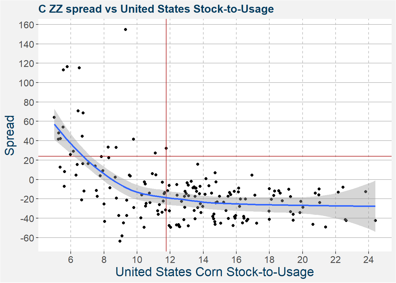
In the case where there is ample supply of a commodity, these supplies have to be carried along the curve to the different delivery months associated with the futures contracts. Since there is a large fee associated with storing a large quantity of the underlying commodity the curve shape will become more contango. There is a theoretical maximum to the degree of contango for any commodity, this is known as full carry and is achieved when all the storage capacity has been filled. For more detail we refer the interested reader to a post on writing calendar spreads as a percentage of full carry. A number that summarises the balance sheet of a major producing nation is stock-to-usage. As its name suggests it is defined as the ratio of ending stock to usage. When this number is high (low) there is ample (insufficient) stock. Intuitively we expect to see a decreasing spread with increasing stock-to-usage. Fundamentally we also expect this effect to become smaller with increasing stock-to-usage where the spread approaches the fully carry value as the stock-to-usage approaches infinity. This behaviour is characteristic of exponential decay. The plot below confirms our intuition. The current values of the WASDE stock-to-usage and C ZZ spread (Corn Dec1 vs Corn Dec2 spread) is indicated by the vertical and horizontal lines respectively. The blue curve with shadow shows a loess fit to the underlying data.
The convenience yield is the benefit or premium associated with holding an underlying physical commodity rather than the associated futures contract. This is closely related to the shape of the futures curve. There are many different ways to define convenience yield mathematically. One approach we like is that of Wei and Zu, who define the convenience yield as \[ y_t = (1 + r) P_{\text{spot}} - P_{t}. \] Where \(r\) is the risk-free rate, \(P_{\text{spot}}\) is the spot price and \(P_t\) is the price of futures contract with expiry \(t\). In words, the convenience yield is the difference between compounding the current spot price at the risk free rate and the further dated futures contract. When the curve is in backwardation the convenience yield is positive. The greater the degree of backwardation the higher the convenience yield.
Hedging pressure is best explained with an example. Broadly, we can distinguish between markets that provide a hedge for producers (backwardated markets) and markets that provide a hedge for consumers (contangoed markets). A commodity producer, such as Exxon, whose business requires it to be long oil, can reduce exposure to oil price fluctuations by being short crude oil futures. In this way, hedging by a risk-averse producer causes futures prices to be below the expected spot rate in the future. On the other hand, a manufacturer such a Boeing is a consumer of aluminium, so it is short aluminium and can reduce the impact of aluminium price fluctuations by purchasing aluminium futures. Hence, hedging by a risk-averse consumer causes futures prices to be higher than the expected spot rate in the future. In these examples, Exxon is willing to sell oil futures at an expected loss and Boing is willing to purchase aluminium at an expected loss. Hedging pressure can be gauged by studying the commitment of traders reports published weekly by the CFTC.
In the following, we consider an example of a bull and bear spread.
4.1.1 Bull Spreads
If we belive that the spread
\[ S = P_{\text{near dated}} - P_{\text{far dated}} \] is going to increase over time we want to have long exposure in a near dated and short exposure in a far dated futures contract. This type of calendar spread structure is called a bull spread.
The perfect time to enter a bull spread is when the curve is trading close to full carry and you have forecasted possible supply shortages in the next season. In this case, the downside is well defined from a fundamental point of view with a big possible upside. Consider the Corn Dec1 vs Corn Dec2 spread above. From the image, we can make a good guess that full carry will be around -50 cents. Assume the current season stock-to-usage numbers are in the mid-teens with a spread of -40. If we are forecasting a possible decrease to sub 10 stock-to-usage we can see the spread increasing to -20 or even larger. In this case, we have a 10 cent downside and a 20 cent upside. This is exactly the type of calendar spread we like to put on.
In the majority of cases the prevailing spread will not be that close to full carry, so an additional amount of risk has to be allowed for. This increase in risk implies that a smaller notional position will be taken to achieve the same risk target. However, the trade still has to give an asymmetric risk-reward profile to be placed on our shortlist.
Another interesting method to profit from a spread trading close to full carry is to make use of spread options. As an example, suppose a calendar spread is trading 10 cents away from full carry and we sell a put spread option for 5 cents. In this case, the downside is only 5 cents, the difference between the distance to full carry and the premium received for the put option. The ideal case is where the premium received pushes the spread past full carry, in this case, the trade has almost zero downside.
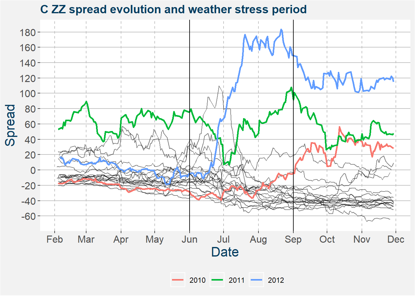
To illustrate a couple of examples from the corn market where bull spreads would have been profitable we consider the image below. The weather stress period lies between the two vertical lines. It is during these times that bull spreads can be extremely profitable. Notice the asymmetric return vs risk over the weather stress period when compared with historical spread during less uncertain weather periods.
4.1.2 Bear Spreads
If we believe that the spread
\[ S = P_{\text{near dated}} - P_{\text{far dated}} \] is going to decrease over time we want to have short exposure in a near dated and long exposure in a far dated futures contract. This type of calendar spread structure is called a bear spread.
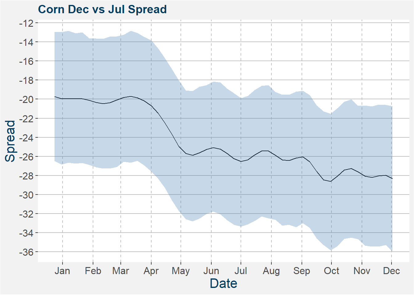
Under normal conditions, without any supply shocks, most agricultural commodities curves will trade more contango into expiry. Below we show the seasonal behaviour of the Corn Dec vs Jul spread. These results were produced with Facebook’s Prophet API. For more information on how the seasonal behaviour of different spreads are determined we refer the interested reader to a write-up on Calendar Spread Seasonal Entries and Exits. The black line shows the mean seasonal spread while the blue shadow represents one standard deviation above and below the mean. Notice how the spread dips into contango from April to May. May through to August is the weather stress period for corn, this coincides with a horizontal motion on average. After the uncertainty in the weather-season has passed and the market becomes more clear on the expected stocks after the harvest we see the curve closing down more contango. Additionally, under normal circumstances, you might be able to squeeze some more out of the steepening of the curve by rolling the short front leg up the curve before expiry.
Bear spreads can be risky over the weather stress periods of different agricultural commodities. There are a couple of ways to mitigate some of this risk. The simplest is to overweight the long leg of the bear spread. Another method uses optionality by buying call options on the near dated part of the curve and selling the call after the weather stress period. For more information on this method, the reader is referred to a post entitled Bear Spread with Call.
We have found that weather-sensitive commodities all show similar behaviour around key weather periods. During these times futures prices and spreads tend to be systematically overvalued because of the uncertainty in upcoming weather. During most cases, an investor would have been profitable trading bear spreads. However, if a bad weather event does materialise, for example during 2012, you need to understand the associated risks and size the position in your portfolio accordingly.
4.2 Inter-Commodity Spreads
As the name suggests, inter-commodity spreads, are trades where we take opposing positions in two fundamentally linked commodities. In essence, we are placing a bet on the direction of the spread between the two (or more) commodities. We write the spread of commodity 1 vs commodity 2 as
\[ S = P_{\text{commodity 2}} - P_{\text{commodity 1}} \] where \(P_{i}\) denotes the futures price of commodity \(i\). In the inter-commodity spread space, we can broadly define two classes of trades, convergence and divergence trades. We investigate each of these below.
4.2.1 Convergence Trades
Convergence trades occur when the spread is suppressed or stretched and we believe that, given the current fundaments, the spread should revert to a more normal range. Below we consider two examples of convergence trades.
Suppressed Process Margin
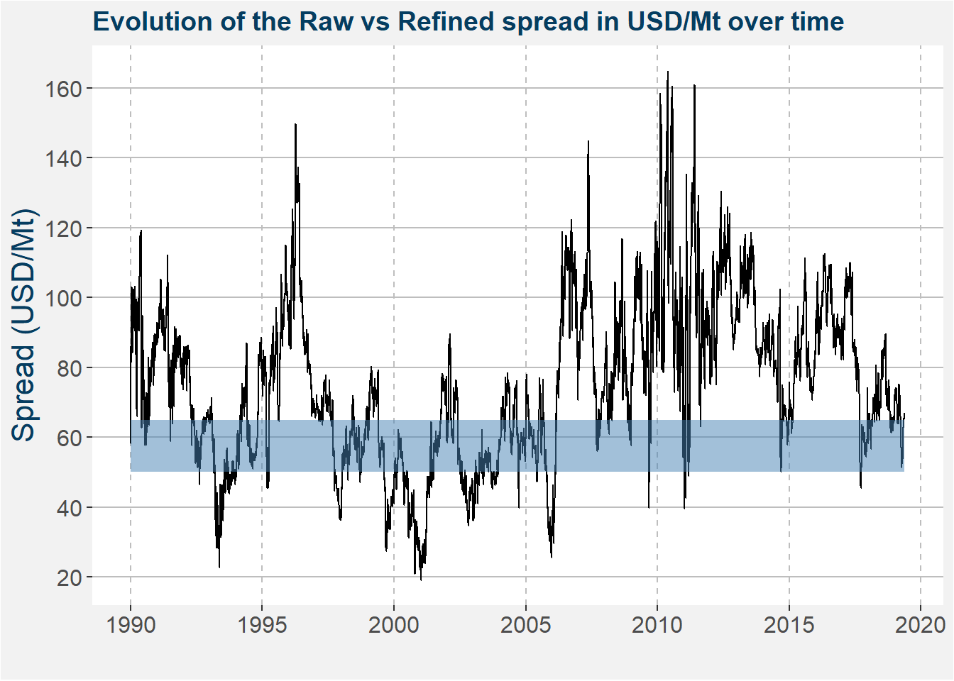
Take for example the raw vs refined sugar process margin trade. Raw sugar in the form of sugar cane or beets has to be refined to get the normal white sugar we are all used to. In the Sugar Trading Manual - Cost of production the author adds a fixed cost of USD 65/t which equates to their estimate of the world average cost of upgrading raw sugar to refined sugar in autonomous refineries.
In the following decrease this cost down to USD 50/t to create a price range where processors will find it difficult to create a profit from refining raw sugar. The plot below shows the time evolution of the SB vs QW spread since 1990. This high-pressure region of USD 50-65/t is highlighted by the blue shaded region.
Below we represent the same data as above in the form of a histogram. The high-pressure processing margin region is highlighted in blue. Superimposed on top of the histogram we show lines representing the 25th, 50th (median) and 75th percentiles together with the values given by the text centered over the lines. Notice that the pressure region coincides with the 25th percentile.
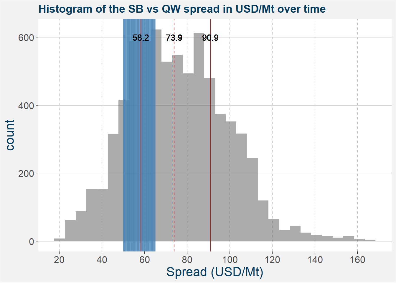
We are interested in this trade when the raw vs refined spread is below USD 55. Here your sugar refineries will be hard-pressed to turn a profit. The lack of refining will force raw sugar supplies to increase. This causes a decrease in the raw sugar price and forces the raw sugar curve to become more contango. Similarly, the lack of refining causes decreases in the refined sugar stock which forces the prices upward and pushes the refined sugar to become more backwardated.
To extract a profit from such a scenario we take up long exposure in refined sugar (QW) and short exposure in raw sugar (SB). This trade behaves particularly well because of the favourable curve structure that arises in these situations. When the short position is in contango and the long position is backwardated you can generate a positive roll return by just holding the trade. If there is a normalisation in the processing margin then this trade gains from the correction in the spread as well as the return from rolling the position forward.
From the Driver of long-term returns section and references therein, it should be clear that the nature of the curve structure plays a prominent role in the returns of the underlying commodities. The roll-adjusted price series give a good indication of the effect of the curve structure.
When forming the roll-adjusted price series we make use of the Panama method where we linearly shift the historical prices upwards in the case of a contango roll and downward in the case of a backwardated roll. We prefer to use a backward adjusted rolled price series such that the front end of the curve overlaps for the adjusted and unadjusted time series. When the curve has had sustained periods of backwardation the cumulative roll adjusted curve has a positive (bottom left to top right) slope. The converse holds when the curve is in contango. Consider the top facet in the plot below showing the price data for refined sugar (QW). Notice that the cumulative roll adjustment curve has a positive slope for the majority of times. Hence the futures curve was in backwardation for the majority of times. This forces the roll adjusted price downward by a value equal to the cumulative roll adjustment at each timestep. The plot below shows the unadjusted and roll adjusted prices in blue and green respectively. The cumulative roll adjustment is given by the red curve. These cumulative values make up the cumulative sum of the discontinuities or jumps in the futures price series when we roll forward.
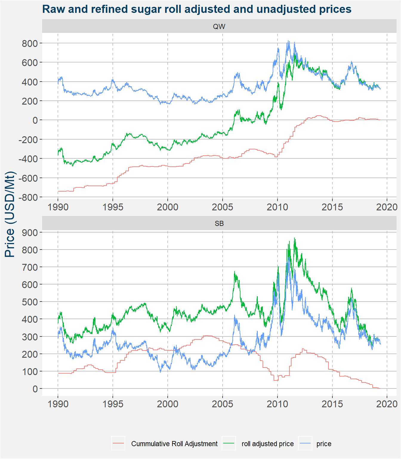
The cumulative roll adjusted values for the raw sugar price data shown in the bottom facet has a mixture of positive and negative slopes, however, the general trend is downward. This downward trend implies the curve must have been in contango for prolonged periods. This cumulative roll adjustment forces the roll adjusted prices upward. This can be seen in the bottom facet of the plot above by the green curve being higher than the blue curve. Notice that the magnitude of the cumulative roll adjustments for QW is much greater than that of SB. This implies that QW will have a much greater impact on how the structure rolls forward.
For more detail on this we direct the interested reader to this white paper the Campbell & Company published in the hedge fund journal.
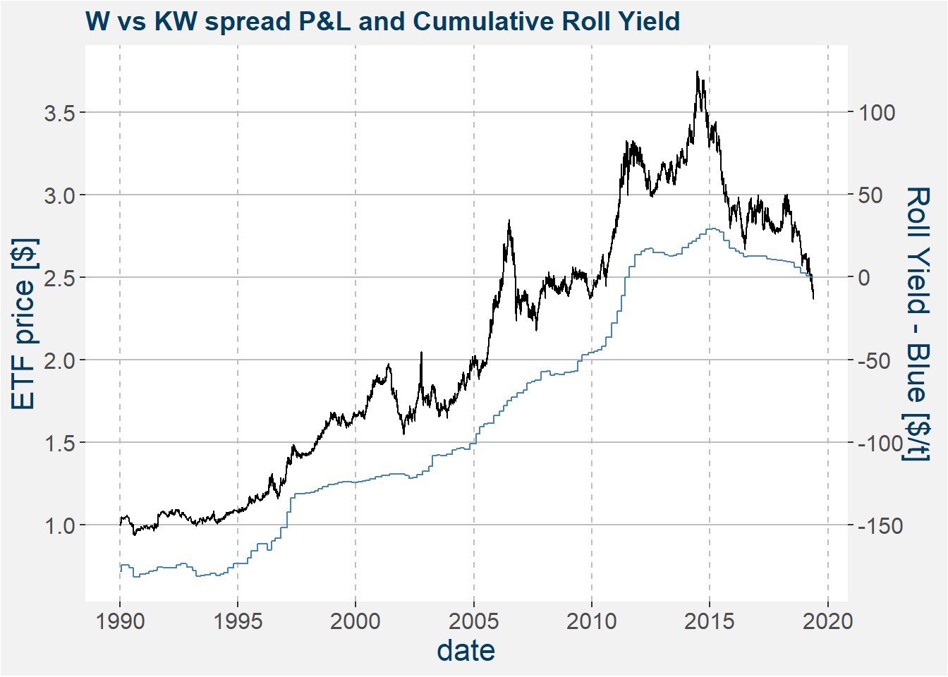
In the plot below we show the value of a USD 1 investment since January 1990 in the raw vs refined sugar spread. Throughout we assume a long position in refined and a short position in raw sugar. Because of the size of the underlying contracts, we trade the spread in a one-to-one ratio. The black line in the plot below shows the value of the USD 1 investment. We do not include trading costs or slippage in the calculations below. The blue curve shows the difference in cumulative roll adjusted values of raw and refined sugar. We define this quantity as the roll yield.
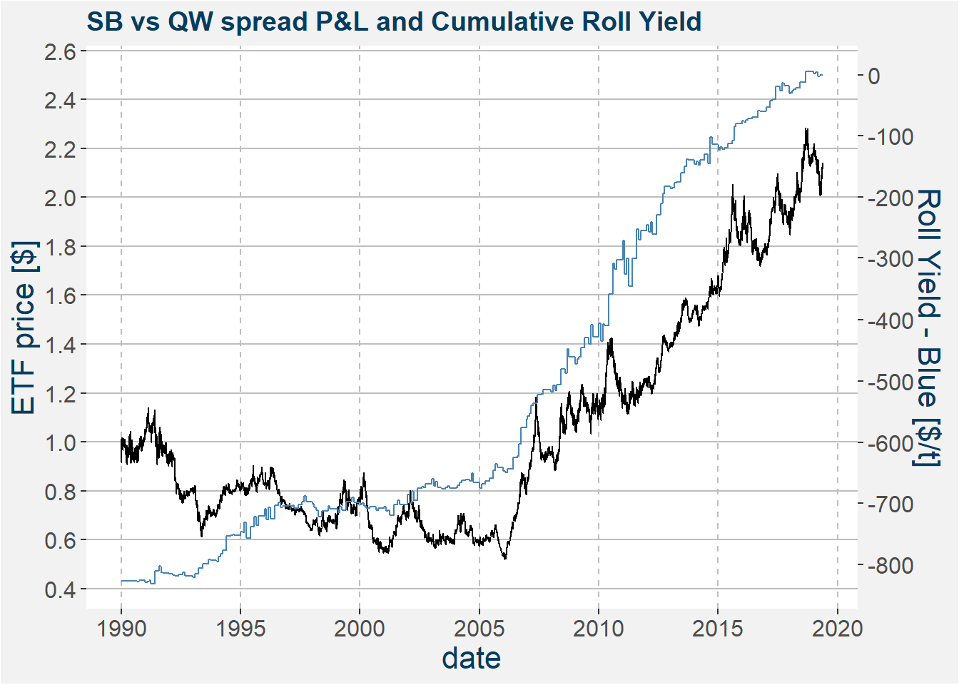
Notice that the form the $1 investment roughly follows the shape of the roll yield. We postulate that the long term return profile of any fundamentally paired relative value spread is directly proportional to the roll yield as defined above. The oscillations about this trend arise from the movement in the spread itself. If these oscillations in the spread outweigh the possible gains from the roll yield a long position in the spread, i.e. long QW and short SB, does not make sense.
If we can forecast the supply and demand of raw and refined sugar we will have a good idea what the curve structures of the two commodities will do. This, in turn, allows us to determine the roll yield given our forecast of the underlying fundamentals. If the roll yield is positive and the spread is trading at suppressed levels it signals a good time to enter this trade. The major form of risk in this type of trade is the term structure of the two commodities. For this reason, we stress the fundamentals in such a way that the curves give negative roll yields over a production cycle. The magnitude of this negative roll yield is then used to size up the position according to the risk target we are comfortable with.
Suppressed Quality Premium
Their is a quality premium that normally arises for wheats containing a greater quantity of protein. Below we show shows where the six main types of wheat are produced in the United States.

Image from www.uswheat.org
Hard red winter (KW) and hard red spring wheat have a higher protein content compared to soft red winter (W) wheat. These higher protein wheats are more versitle and produce higher quality baked goods. For this reason we expect to see, on average, a premium for the wheat with a higher protein content. The image below confirms this intuition. The vertical line shown the zero marker, below which, the high protein wheat trades at a discount to the lower protein wheat.
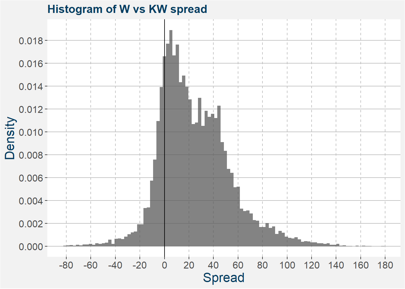
When the high protein wheat (KW) it trading at a discount to the low protein wheat (W) it signals a good time to enter this trade. In this case the high protein wheat stocks will decrease because of the discount. This reduction in stock will force the high protein wheat curve less contango. Conversely, the stocks of the low protein wheat will build forcing the curve more contango. To extract a profit from such a scenario we take up long exposure in the high protein (KW) wheat and short exposure in the low protein wheat (W). Under these conditions the we should see a positive roll yield because the short leg is rolled at a steeper contango compared to the long leg.
The plot below shows the value of a USD 1 investment in the spread since January 1990. Throughout we assume a long position in high protein wheat and a short position in low protein wheat. These contracts have similar size, so we trade this spread on a one-to-one basis. The black line shows the value of the USD 1 investment. We don’t include trading costs or slippage in the calculations below. The blue curve shows the difference in cuulative roll adjusted values of the high and low protein wheats. Similar to the raw vs refined sugar case we see that the roll yield domonates the long-term performance of the spread.
We follow a very similar process to identify entries for other types of convergence trades, which include
- Substitution
- Geographical Arbitrage
- Crack spreads
The steps can be summarised as:
- Obtain a universe of fundamentally linked groups of commodities
- Within each group, find a fundamental reason why certain commodities trade at a premium or discount
- When the spread is suppressed or stressed we add the trade to our shortlist
- Forecast and stress the fundamentals to determine the downside risk in the spread and roll yield
- Determine reward vs risk
- Given a flat or positive roll with an asymmetric reward vs risk profile we include the trade in our execution list
- Size trade up with 1% of NAV convention
- For higher conviction trades we size up slightly larger.
4.2.2 Divergence Trades
Divergence trades most often arise from forecasted breaks in the supply and demand dynamics of the major producing and consuming nations for each of the commodities.