1 Introduction
The aim of this write-up is to give some proof of principle results on extracting P&L from the difference in roll yield between two correlated commodities. We define the roll yield as the daily compound return that changes the further dated contract price to the near dated contract price. Mathematically we write
\[ Y^a_{i,j} = \left[ \left( \frac{P^a_i}{P^a_j} \right) ^ {1/N^a_{i,j}} - 1 \right] \times 100 \] Here, \(P^a_i\) denotes the price of commodity \(a\) with expiry \(i\). We assume \(j > i\), i.e. contract \(j\) expires after contract \(i\). Finally we define \(N^a_{i,j} = |i-j|\) as the number of days between expiry of contracts \(i\) and \(j\) for commodity \(a\).
When the curve is in backwardation, i.e. \(P^a_i > P^a_j\), we see that the roll yield \(Y^a_{i,j}\) is positive. This positive number is the percentage increase by which the deferred contract has to increase in order to have the same price as the front contract on expiry. Similarly, when the curve is in contango, i.e. \(P^a_i < P^a_j\), the roll yield is negative and the number can be interpreted as the daily percentage decrease to take the deferred price to the front price at expiry of the front contract.
We group our universe of commodities into six categories,
- Agri (12),
- Base Metals (6),
- Precious Metals (4),
- Softs (6),
- Meats (4) and
- Energies (6).
The numbers in brackets indicate the number of commodities included in that group. The different groups are shown in the table below. Here a 1 indicates that the commodity, in each row, is included in the category, in each column. Some commodities may be present in multiple groups. We group the commodities into different categories to avoid comparing the roll yield between pairs that do not make fundamental sense, for example comparing the roll yields of gold (GC) and corn (C).
| Agri | Base Metals | Energies | Meats | Precious Metals | Softs | |
|---|---|---|---|---|---|---|
| BO | 1 | NA | NA | NA | NA | NA |
| C | 1 | NA | NA | 1 | NA | NA |
| CA | 1 | NA | NA | NA | NA | NA |
| CC | NA | NA | NA | NA | NA | 1 |
| CL | NA | NA | 1 | NA | NA | NA |
| CO | NA | NA | 1 | NA | NA | NA |
| CT | 1 | NA | NA | NA | NA | NA |
| DF | NA | NA | NA | NA | NA | 1 |
| FC | NA | NA | NA | 1 | NA | NA |
| GC | NA | NA | NA | NA | 1 | NA |
| HG | NA | 1 | NA | NA | NA | NA |
| HO | NA | NA | 1 | NA | NA | NA |
| KC | NA | NA | NA | NA | NA | 1 |
| KO | 1 | NA | NA | NA | NA | NA |
| KW | 1 | NA | NA | NA | NA | NA |
| LA | NA | 1 | NA | NA | NA | NA |
| LC | NA | NA | NA | 1 | NA | NA |
| LH | NA | NA | NA | 1 | NA | NA |
| LL | NA | 1 | NA | NA | NA | NA |
| LN | NA | 1 | NA | NA | NA | NA |
| LT | NA | 1 | NA | NA | NA | NA |
| LX | NA | 1 | NA | NA | NA | NA |
| MW | 1 | NA | NA | NA | NA | NA |
| NG | NA | NA | 1 | NA | NA | NA |
| PA | NA | NA | NA | NA | 1 | NA |
| PL | NA | NA | NA | NA | 1 | NA |
| QC | NA | NA | NA | NA | NA | 1 |
| QS | NA | NA | 1 | NA | NA | NA |
| QW | NA | NA | NA | NA | NA | 1 |
| RR | 1 | NA | NA | NA | NA | NA |
| RS | 1 | NA | NA | NA | NA | NA |
| S | 1 | NA | NA | NA | NA | NA |
| SB | NA | NA | NA | NA | NA | 1 |
| SI | NA | NA | NA | NA | 1 | NA |
| SM | 1 | NA | NA | NA | NA | NA |
| W | 1 | NA | NA | NA | NA | NA |
| XB | NA | NA | 1 | NA | NA | NA |
Using the construction outlined above we have 123 different pairs. The number of different pairs withing each category is shown in the table below. For each of these pairs we determine the relative roll yield. We take long exposure to the commodity the greater roll yield and short exposure to the commodity with smaller roll yield.
| pairs | |
|---|---|
| Agri | 66 |
| Base Metals | 15 |
| Precious Metals | 6 |
| Softs | 15 |
| Meats | 6 |
| Energies | 15 |
| Total | 123 |
2 Explore the Roll Yield
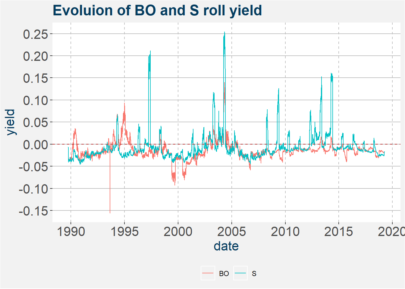
The plot below shows the evolution of the bean oil and soybean roll yield. The horizontal dashed red line indicastes the zero mark. Negative roll yield imply the curve was incontango and positive roll yields imply it was in backwardation. In the case of the BO vs S pair we take up long expossure to the commodity with the greater roll yield and short exposure to the commodity with the lower roll yield.

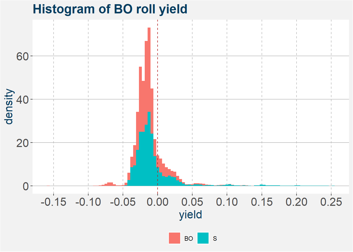
This negative roll yield in bean oil is emphasised in the histogram below together with the rol yield of soybeans. The majaroty of the bars lie below the zero line given by the vertical dashed red line.

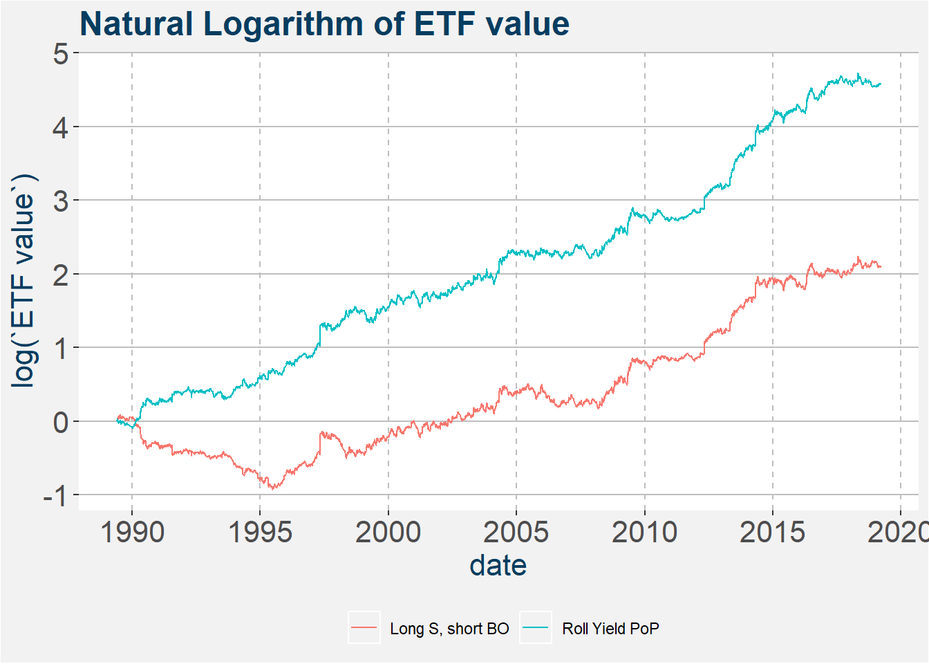
The plot below shows the the value of a $1 investment in the BO vs S spread (long S, short BO) and the proof of principle (PoP) results where the change the long exposure to the commodity with the greater roll yield. Note that the proof of principle result does not include any fees.

3 Simple Model
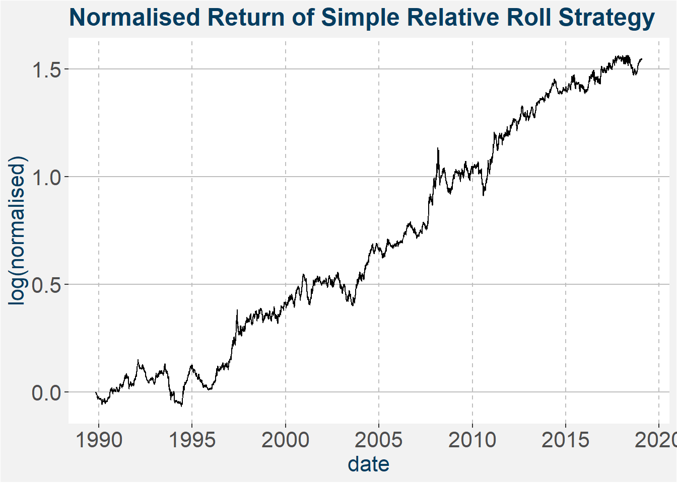
Here we consider a very simple model. For each of the commodities we detremine the roll adjusted price series and find the roll dates. We define the roll dates as the roll yield calculation dates. On these dates and for each pair we take long exposure to the commdity with greater roll yield. We assume a USD 10 futures round trip cost and pay away a tick on each side of the trade. For each pair we allocate 1/123 of NAV where the contract with the smallest notional amount fills the alloted amount to the nearest integer. Long and short legs are traded in equal numbers of contracts. The plot below shows the value of a $1 investment in this strategy. The table belwo the graph gives some performance statistics.

| Relative Roll | |
|---|---|
| Annualized Return | 5.260 |
| Annualized Std Dev | 8.610 |
| Annualized Sharpe (Rf=0%) | 0.612 |
| Maximum Drawdown | 20.113 |
| Maximum Drawdown/Annualized Return | 3.824 |
| Number of Positive Months | 207.000 |
| Number of Negative Months | 145.000 |
| Average Positive Month Return | 2.035 |
| Average Negative Month Return | -1.761 |
4 Comments
This is just a simple proof of principle model and gives promising results. There are a number of ways we can try to enhance the model’s performance. These will be added in subsequent posts.