Introduction
In this write-up, we explore how the front month price and time to expiry of the front-month contract can be used to model the C UZ spread.
Seasonalality
Using a similar methodology to the Calendar Spread Seasonal Entries and Exits post, we study the roll adjusted seaonal behaviour of the C UZ spread.
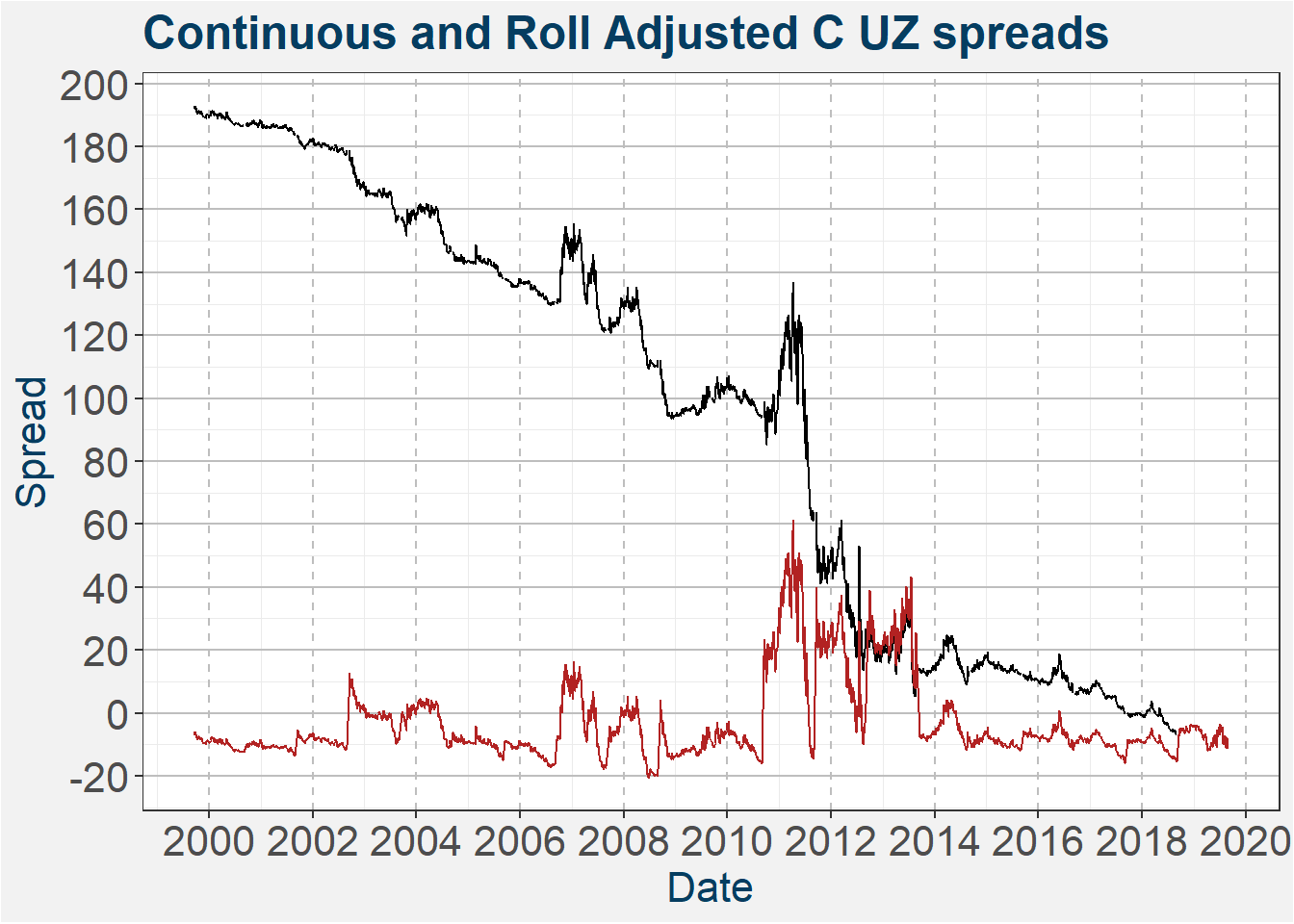
The plot below shows the continuous and roll adjusted C UZ spreads since 2000. Notice that only during the extreme weather events did the spread backwardate.
It is interesting to note the behaviour of this spread as a stand-alone strategy. Below we show the cumulative return of a portfolio made up entirely of short exposure to C UZ since September 1999. Here we assume we are fully employed on a notional level on the long and short legs of the spread. Transaction costs and slippage have also not been included. As we saw above the main drawdown periods coincide with the weather stress the United States experienced from 2011 through 2013.
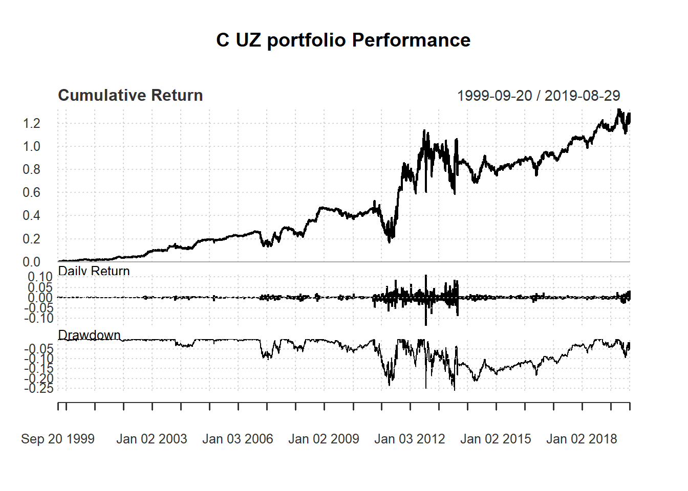
The table below summarises the performanca statistics of this strategy.
| C UZ portfolio | |
|---|---|
| Annualized Return | 0.0443 |
| Annualized Std Dev | 0.1382 |
| Annualized Sharpe (Rf=0%) | 0.3205 |
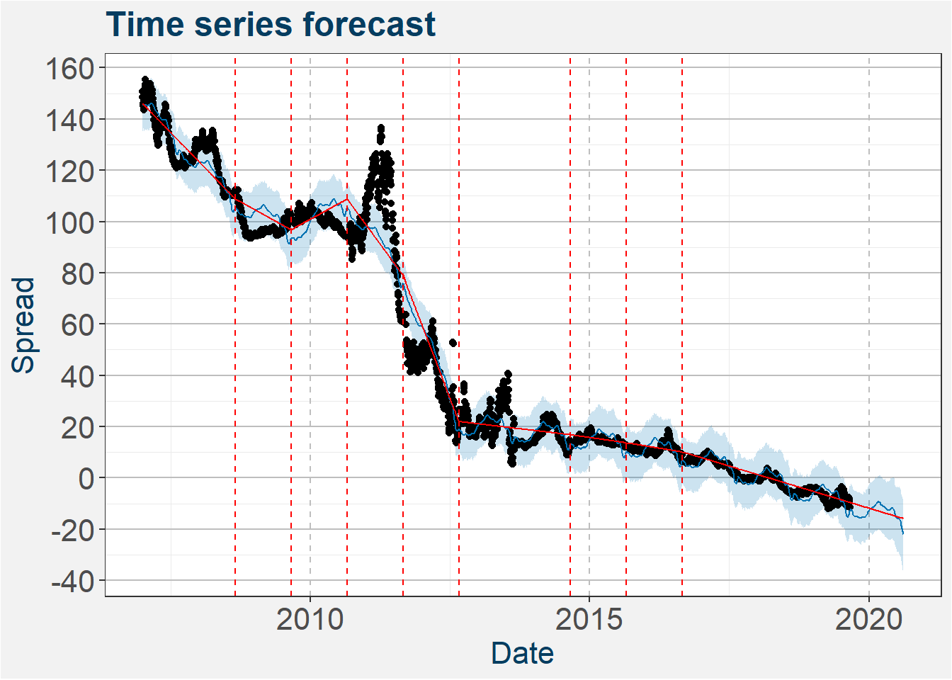
From the rolled spreads we determine the forecasted spread using time-series decomposition where we strip out the seasonal and trend behaviour of the time-series. The model results are shown in the plot below. The vertical dashed red lines show the trend turning points.
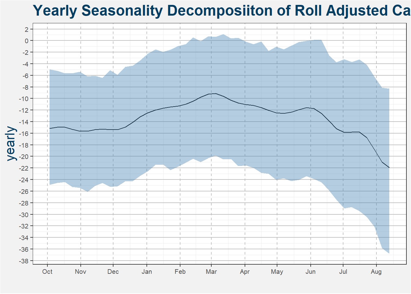
The plot below shows the mean seasonal and trend of the C UZ spread. From October through March we see a 5 cent increase followed by a 5 cent decrease going into expiry of the C U contract. Note that there reflect the average behaviour of the spread.
Spread vs Front Month
We know the front month will play a major part in the value of the spread purely by the defition of the spread
\[ S_{\text{UZ}} = P_{\text{U}} - P_{\text{Z}} \] where \(P_{\text{i}}\) if the price of contract \(i\). In the plot below we try to determine some critical price value that splits the (price, spread)-space into distinct parts. In this case, we use a simple k-means clustering algorithm similar to the one used in this write-up. Notice that the behaviour of the spread is quite different for the two regions. We can say that for front-month prices above the USD 5 mark we tend to see the spread increase.
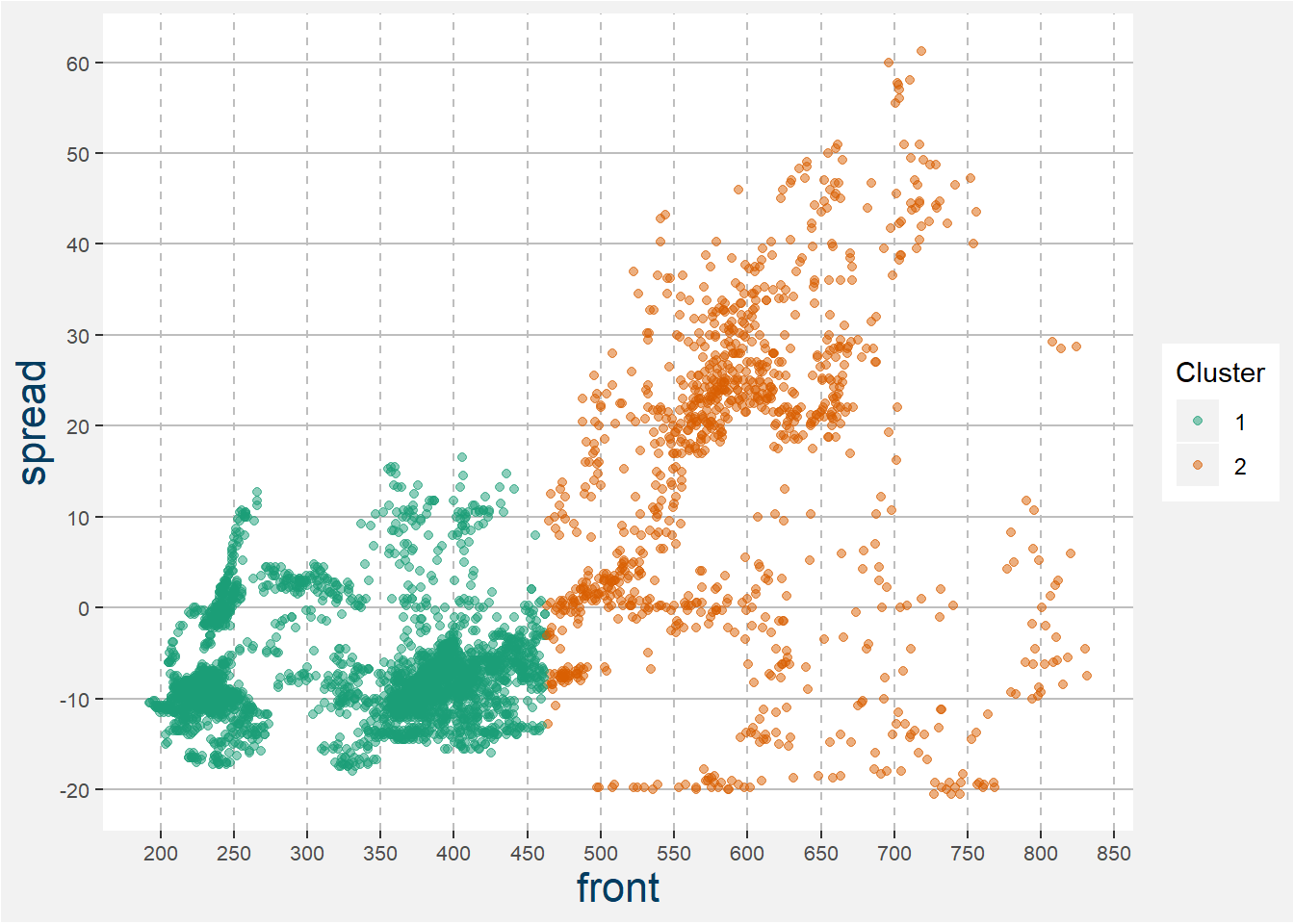
From the first section, we saw that there is a clear seasonal component in the C UZ spread and that this spread like to trade more contango going into expiry. In the following section, we combine the time to expiration and front-month price to add a temporal dimension to modeling the value of the spread.
Spread Evolution Model
We used a kNN model cross-validated and hyperparameter tuned on each of the available front contract years. As input features, we use the normalised values of the front-month price and days to expiry. The image below summarises the results of the model. On the y-axis, we show the predicted value of the spread. The x-axis shows the number of days until the expiry of the contract. The slider can be used to select a front month price.
Another way to view this data is as a heatmap. In the plot below the more yellow (blue) the more backwardated (contangoed) the spread. Time is represented by the x-axis and should be read from left to right. In realy all cases the predicted spread becomes more blue as time progresses toward expiry.
Remarks
Two premias are up for grabs in the spread
- Carry and
- Weather risk.
This is a spread with strong seasonal trends toward increased contango as we move close to expiry. During weather stress periods there is an opportunity on the upside, but even under stressed conditions, the spread tends to close out lower going into expiry.