Introduction
In this write-up we study the historical optimal hedging ratio for the KW vs CA spread. This work follows from previous research on the optimal hedging ratio of the C vs S spread.
The table below gives the contract specifications of KW and CA. Notice that the tons per contract is basically equivalent, i.e. when sizing up the positions on a ton for ton basis we make use of a one to one ratio.
| comdty | units | constractsize | pricebasis | tonspercontract | multiplier |
|---|---|---|---|---|---|
| CA | Metric Tonnes | 50 | EUR/Mt | 50.0000 | 50 |
| KW | Short Bushels | 5000 | USd/Sbushel | 136.0791 | 50 |
We are interested in different parts of the futures curves of the inter commodity spread. We use the nomenclature tenor to denote the part of the curve we are interested in. Here, 0 refers to the front most part of the curve we are interested in. The greater the number the further along the curve the relative position will be entered. The table below shows the roll schedules of the different tenors.
| KW | CA | KW | CA | KW | CA | KW | CA | |
|---|---|---|---|---|---|---|---|---|
| January | H | H | K | K | U | U | Z | Z |
| February | K | K | U | U | Z | Z | H | H |
| March | K | K | U | U | Z | Z | H | H |
| April | U | U | Z | Z | H | H | K | K |
| May | U | U | Z | Z | H | H | K | K |
| June | U | U | Z | Z | H | H | K | K |
| July | Z | Z | H | H | K | K | U | U |
| August | Z | Z | H | H | K | K | U | U |
| September | Z | Z | H | H | K | K | U | U |
| October | H | H | K | K | U | U | Z | Z |
| November | H | H | K | K | U | U | Z | Z |
| December | H | H | K | K | U | U | Z | Z |
We define the hedging ratio \(k\) with respect to the spread \(S^{\prime}\) as
\[ S^{\prime} = P_{CA} - k P_{KW} \]
where \(P_{CA}\) and \(P_{KW}\) denote the US Dollar per ton prices CA and KW respectively. In the following we study the hedging ratios \(k\) that would have given the best historical risk adjusted returns from trading the spreads \(S^{\prime}\) on the long side. To measure risk adjusted return we make use of the Sharpe ratio. Throughout we assume for every one long position in CA a short position of \(k\) in KW.
A note on CA data
The European wheat data have undergone a couple of changes over the past where certain contracts have stopped and new ones have started. The table below shows a reduced version of the contracts associated with CA. Notice that the F contract stopped in 2015, while the Q and X contracts stopped in 2012 and 2014 respetively. The U and Z contracts then started in 2015. In order to create a larger historical database for the spreads we associated the X and Z contract with each other. Similarly we associated Q and U with each other.
| year | F | H | K | N | Q | U | X | Z |
|---|---|---|---|---|---|---|---|---|
| 2009 | 1 | 1 | 1 | NA | 1 | NA | 1 | NA |
| 2010 | 1 | 1 | 1 | NA | 1 | NA | 1 | NA |
| 2011 | 1 | 1 | 1 | NA | 1 | NA | 1 | NA |
| 2012 | 1 | 1 | 1 | NA | 1 | NA | 1 | NA |
| 2013 | 1 | 1 | 1 | NA | NA | NA | 1 | NA |
| 2014 | 1 | 1 | 1 | NA | NA | NA | 1 | NA |
| 2015 | 1 | 1 | 1 | NA | NA | 1 | NA | 1 |
| 2016 | NA | 1 | 1 | NA | NA | 1 | NA | 1 |
| 2017 | NA | 1 | 1 | NA | NA | 1 | NA | 1 |
| 2018 | NA | 1 | 1 | NA | NA | 1 | NA | 1 |
| 2019 | NA | 1 | 1 | NA | NA | 1 | NA | 1 |
| 2020 | NA | 1 | 1 | NA | NA | 1 | NA | 1 |
| 2021 | NA | 1 | 1 | NA | NA | 1 | NA | 1 |
| 2022 | NA | 1 | 1 | NA | NA | 1 | NA | NA |
This way we force the CA to only have H, K, U and Z contracts which we combine with the same KW contracts to form the spreads.
Long Term Behaviour
A classic way to trade the KW vs CA spread is on a ton-for-ton basis. This amounts to a hedging ratio \(k = \frac{50}{136} \approx 0.37\). In words, for every 1 lot of CA we require 0.37 lots of KW to trade this spread on a ton for ton basis. The plot below shows the evolution of $1 invested in the spread from 1999. The different colours represent the different tenors. It is clear that the tenors closer to the front end of the curve produce the best returns.
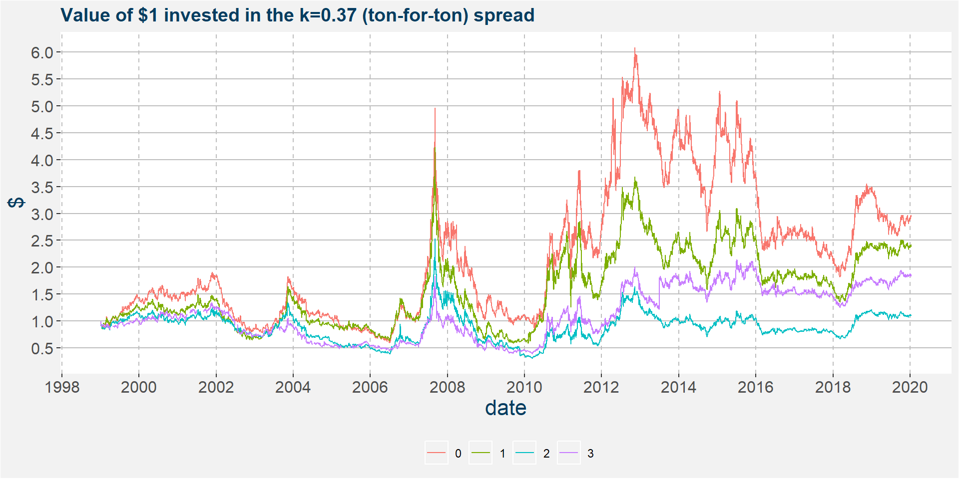
The table below summarises the return statistics of the KW vs CA spread since 1999. Notice that the front end of the curve, tenor 0, gives the greatest annualised return and has the highest Sharpe ratio. Each column represents the different tenors we are interested in.
| 0 | 1 | 2 | 3 | |
|---|---|---|---|---|
| Annualized Return | 0.0530 | 0.0424 | 0.0043 | 0.0308 |
| Annualized Std Dev | 0.4056 | 0.3905 | 0.3866 | 0.3879 |
| Annualized Sharpe (Rf=0%) | 0.1308 | 0.1086 | 0.0110 | 0.0794 |
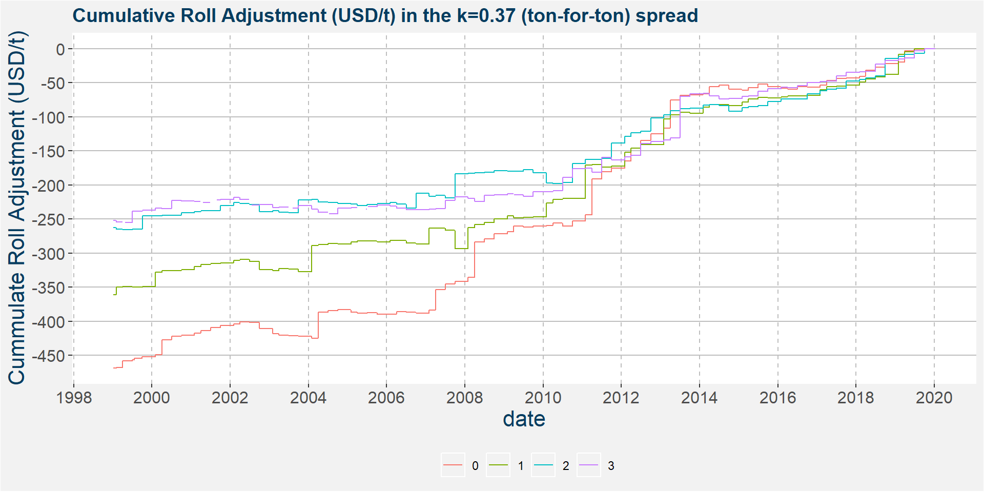
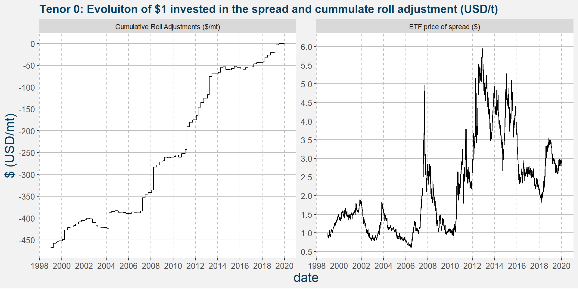
The plot below shows the cumulative roll adjustments in USD/t over the same period as the plot above. Notice that the slopes of the cumulative roll adjustments are positive over the long term, showing a positive roll return on average. When we compare the above and below plots we can see that tenors with the best performance are those that experiences the best roll returns.
Throughout we explore hedging ratios ranging from 0 to 5 with increments of 0.1. The plot below shows the Sharpe ratio of the KW vs CA strategy as a function of the hedging ratio. The optimal Sharpe ratio is obtained when the slope of the graph is zero, ie. the turning point, indicated below by the dashed horizontal and vertical lines. Similar to before the different colours respresent the different tenors. The plots below were constructud using the full sample of data from 1999 to the most recent, hence the optimal hedging ratios are those for the entire duration of the sample.
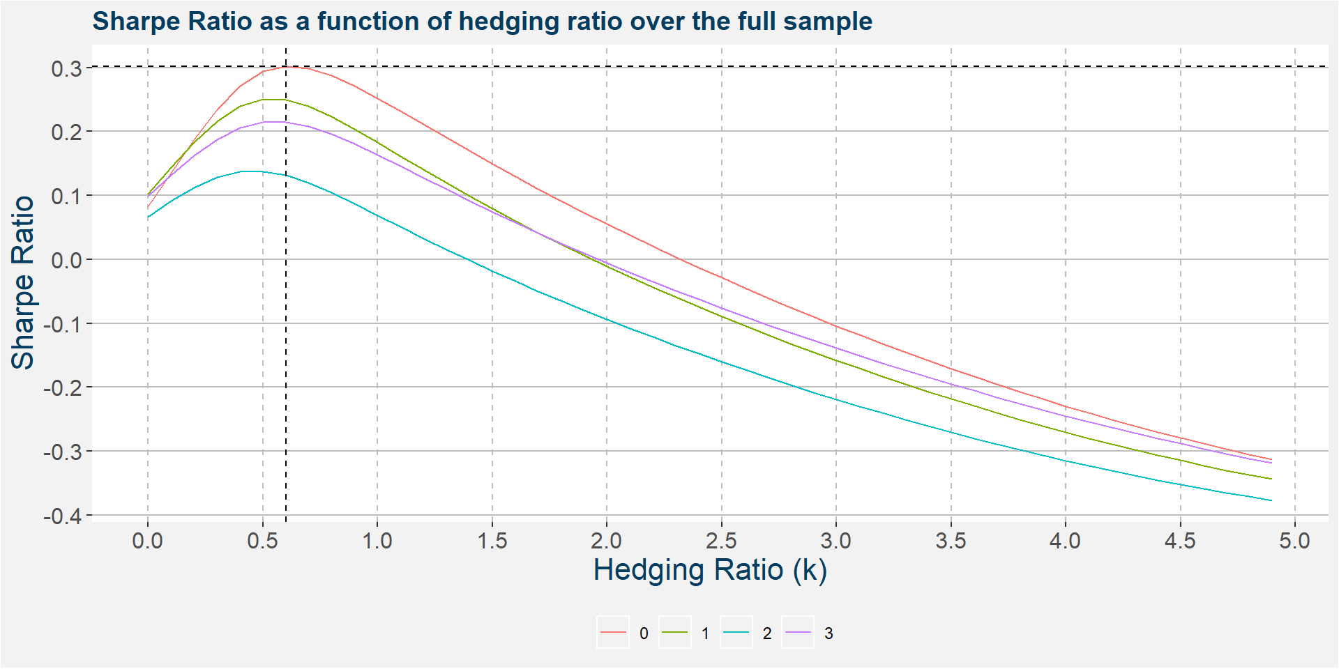
The table below shows the hedging ratios with the optimal Sharpe ratios for each of the tenors. Note that the full sample data gives the best risk adjusted reward with a hedging ratio of around 0.6. The table has columns denoted risk and reward. These amount to annualised standard deviation of returns and annualised return respectively.
| tenor | sharpe | risk | reward | hedging ratio |
|---|---|---|---|---|
| 0 | 0.3018827 | 16.32086 | 4.926985 | 0.6 |
| 1 | 0.2502612 | 14.78919 | 3.701160 | 0.5 |
| 2 | 0.1377372 | 14.66145 | 2.019427 | 0.5 |
| 3 | 0.2150383 | 15.23767 | 3.276683 | 0.6 |
If we compare the Sharpe ratios of the optimal hedging ratio with that of the ton-for-ton case we see that the return is more or less the same, but the risk, as measured by the annualised standard deviation of return, is less than half. Also notice that the optimal hedging ratio is much greater than the corresponding hedging ratio used in the ton-for-ton scenario. In words we can say that for every one lot we are long CA we need to be 0.6 lots short KW. When converting this to tons we see that for every 1 ton we are long CA we need to be short 1.632 tons KW. Note this is to get the optimal risk adjusted return over the entire sample.
Calendar Year Behaviour
Hedging Ratios
In this section we study the calendar year performance of the strategy, i.e. Jan-Dec behaviour. For each calendar year we determine the hedging ratio that yielded the highest Sharpe ratio. The results are shown in the plot below. Notice that thare are a couple of years where the optimal hedging ratio was zero, i.e. only a long position in CA was taken with no offsetting position in KW. Below we only show the results for tenor 0 since the other tenors’ results look similar.
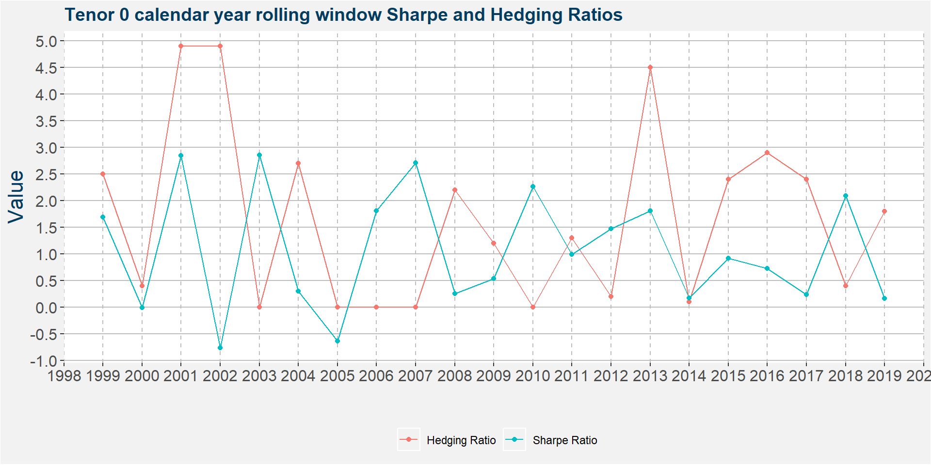
Notice that the majority of calendar years have positive Sharpe ratios. There are also many instances where the optimal hedging ratio was zero. We take a closer look at these cases below. The table below highlights those calendar years where the strategy had a negative Sharpe ratio. From the historical data we see that the 2002 calendar year had the worst performance.
| Hedging Ratio | Sharpe Ratio | tenor | year |
|---|---|---|---|
| 4.9 | -0.7600327 | 0 | 2002 |
| 0.0 | -0.6327121 | 0 | 2005 |
| 0.4 | -0.0082860 | 0 | 2000 |
The plot below shows the evolution of the tenor 0 spread (\(k=0.37\)) during 2002. Notice that the spread increased by $60 during this period.
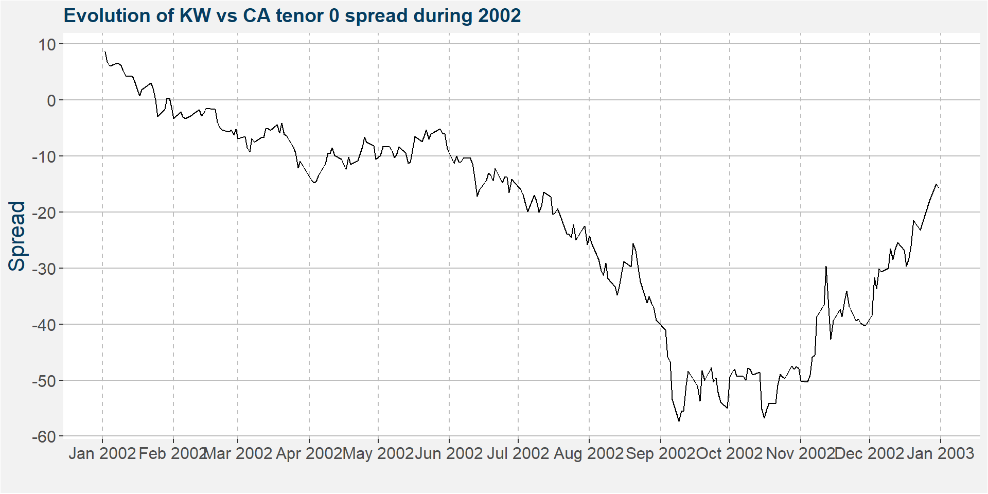
The collapse of the spread above can be attributed to a decrease in the price of CA. The plot below shows the value of $1 invested in each of the commodities on the first business day of 2002.
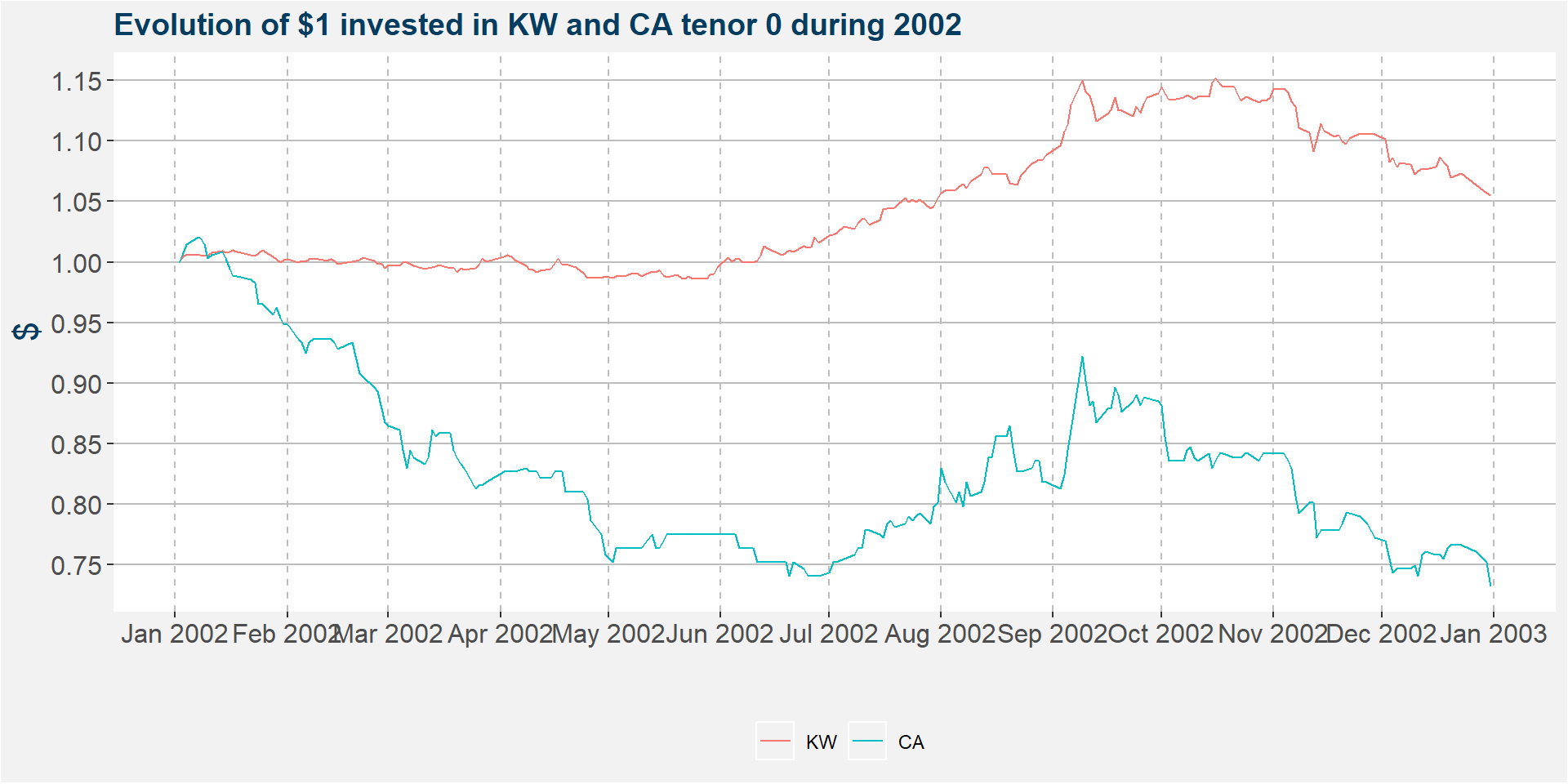
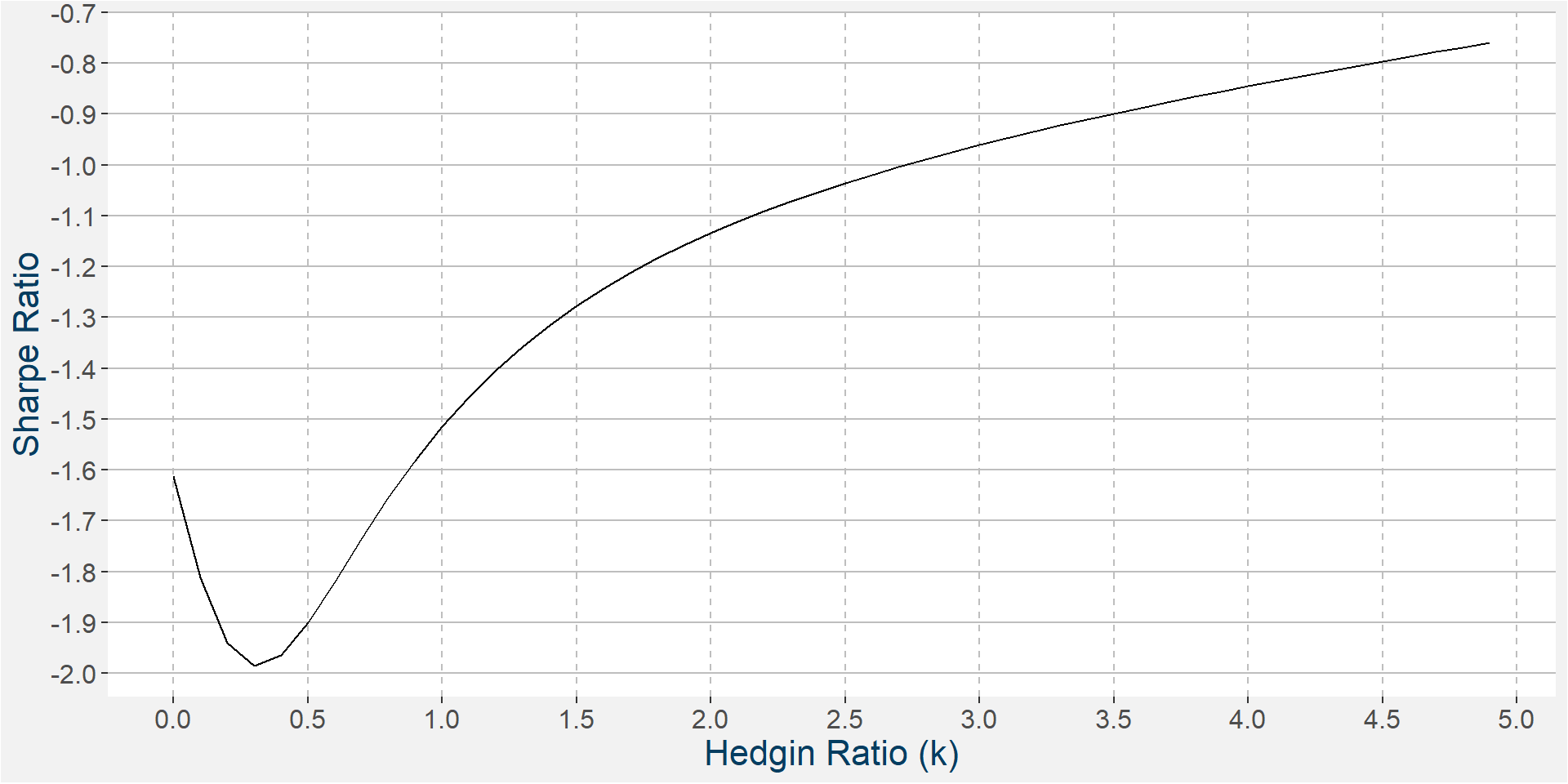
The only way that the hemorage could have been stopped, while being long the spread, would have been to increase the hedging ratio. The plot below shows the 2002 Sharpe ratio as a function of the hedging ratio. Notice that all the Sharpe ratios in the image are negative. The Sharpe ratio does become less negative with increasing hedging ratio.
The table below hightights the results of the cases where the optimal hedging ratio was determined to be zero. Note these are the cases where it would have been best not to take a short KW position. Two cases that stand out, from a positive Sharpe ratio point of view, are the 2003 and 207 calendar years.
| Hedging Ratio | Sharpe Ratio | tenor | year |
|---|---|---|---|
| 0 | -0.6327121 | 0 | 2005 |
| 0 | 1.8061818 | 0 | 2006 |
| 0 | 2.2639610 | 0 | 2010 |
| 0 | 2.7059090 | 0 | 2007 |
| 0 | 2.8510493 | 0 | 2003 |
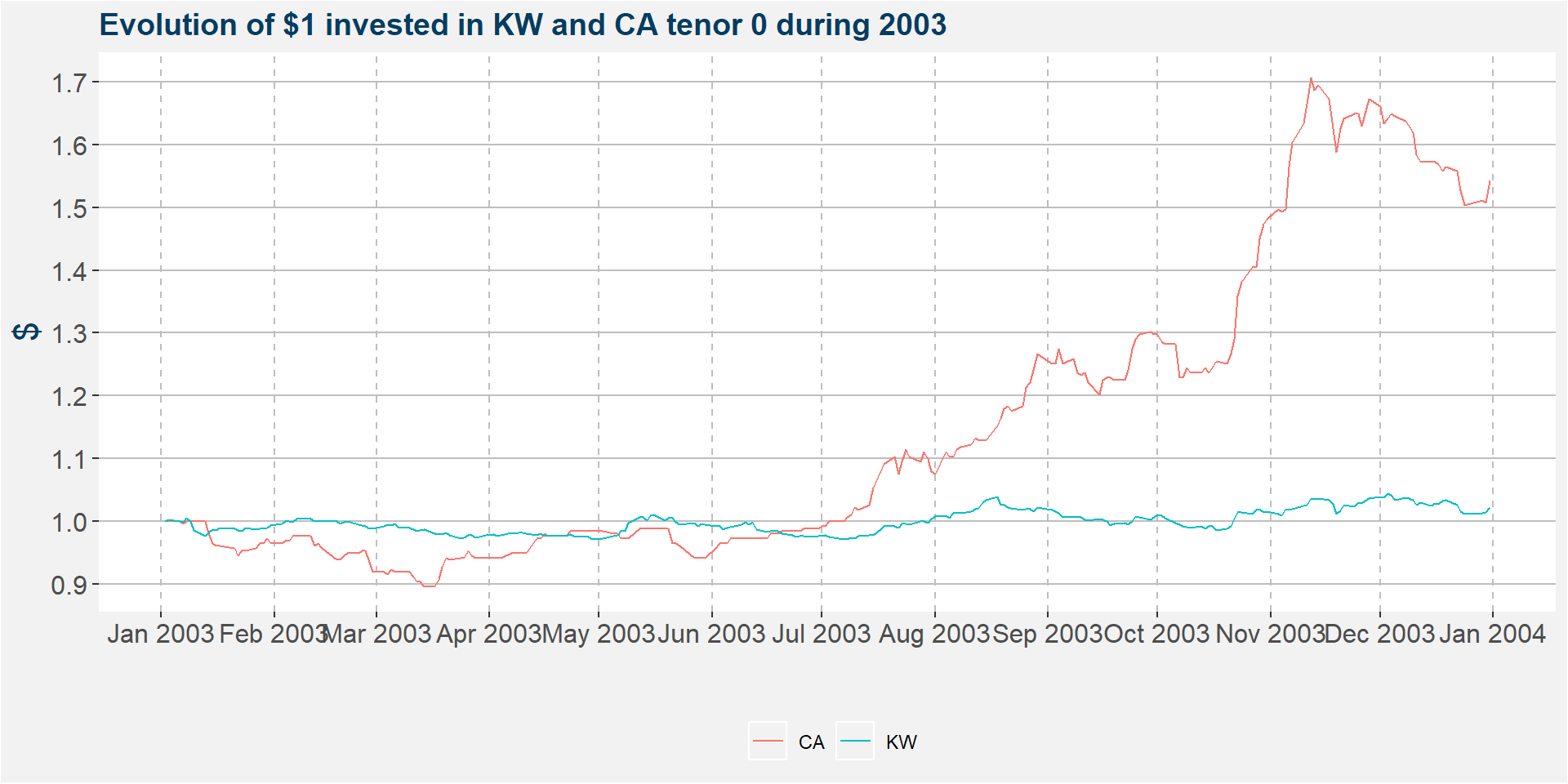
The plot below shows the value of $1 invested in each of the commodities during 2003. Notice that all the returns during 2003 can be attributed to the long position in CA.
The plot below shows the value of $1 invested in each of the commodities during 2007. Here too, the vast majority of the returns are dominated by the long position in CA.
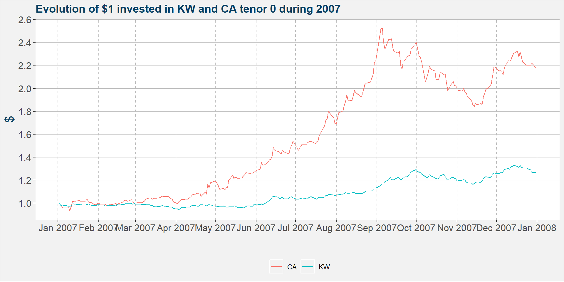
The performance statistics of beying long both of the commodities is given in the table below. Recall that the spread always takes up a long position in CA and a short KW. In this case it is clear that the return from the spread will have given the best results with a hedging ratio \(k=0\) since any short position in KW would have reduced the return from the spread.
| KW | CA | |
|---|---|---|
| Annualized Return | 0.6288 | 0.7622 |
| Annualized Std Dev | 0.2924 | 0.2762 |
| Annualized Sharpe (Rf=0%) | 2.1502 | 2.7600 |
It is interesting to note that the years that gave the largest returns were those were CA dominated the performance. Naturally in these cases a lower hedging ration would have been preferable.
Cumulative Roll Adjustments
A mathematical shorthand for the cumulative roll adjustment can be written as
\[ \text{CRA}_{S,C}(k) = \sum \Delta P_S - k \sum \Delta P_C \]
with
\[ \Delta P_S = P_S(\text{front}) - P_S(\text{deferred}) \] where \(\text{CRA}_{S,C}(k)\) denotes the cumulative roll adjustment with hedging ratio \(k\) between commodities S and C. \(P_S(\text{front})\) and \(P_S(\text{deferred})\) denotes the front and deferred parts of the curve, so that \(\Delta P_S\) is just the standard convention of a calendar spread. The cumulative roll adjustment of the spread can then be understood as the sum over all the calendar spreads of the two commodities over the respective roll periods taking the hedging ratio into account.
The plot below shows the cumulative roll adjustment and the value of $1 invested in the KW vs CA spread since 1999. Notice that the cumulative roll gaps do not form a long term envelope for the long term returns of the spread to the same extent as it does in other spreads. The spread seems to be more dominated by the shorter term price moves of the underlying commodities. The cumulative roll returns are calculated as the difference between the cumulative roll adjustments of the CA and KW futures curves. In the plots below we have set the hedging ratio to \(k=0.37\).
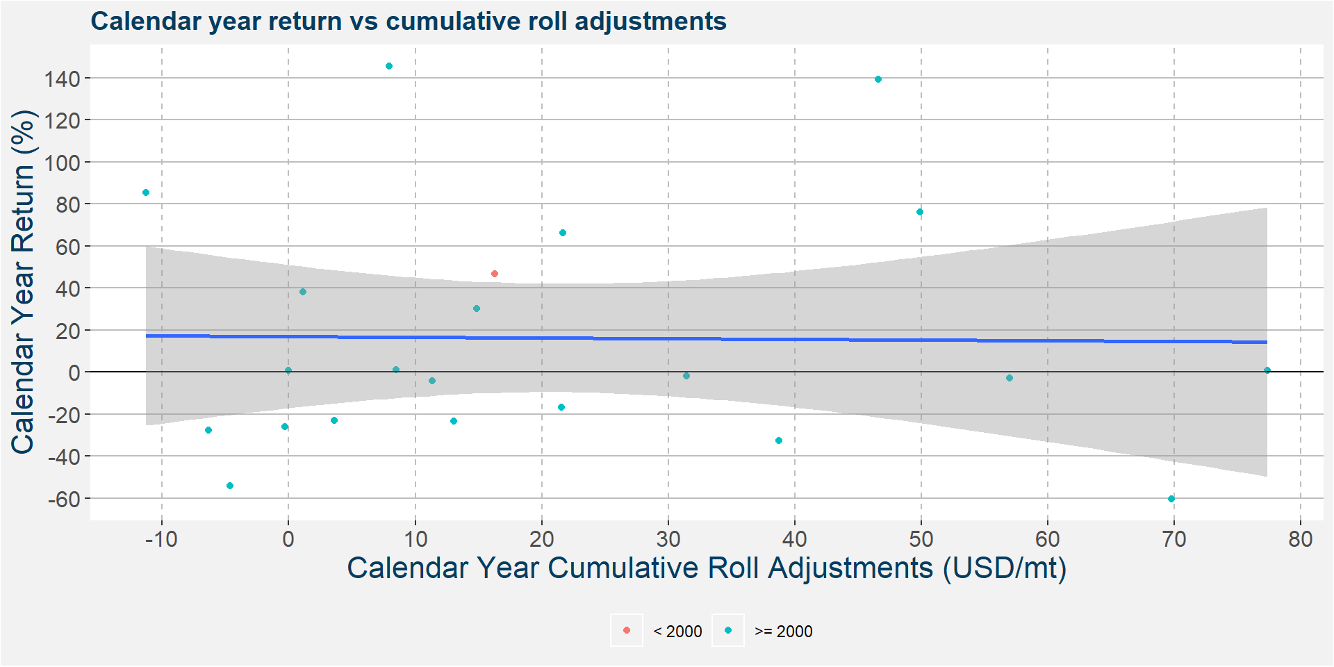
In the plot below we show the calenar year return as a funciton of cumulative roll adjustments. We highlight the zero percentage return line by the solid black line and superimpose a best fit linear regression to the data. Notice that the slope is basically zero implying a near zero correlation between the cumulative roll adjustment and calendar year return.
The table below summarises the calendar year results. The first column groups the calendar year returns with respect to their signs, +1 and -1 for positive and negative returns respectively. The bottom row shows the total for each of the columns. The values under the Cumulative Roll Adjustment heading show the number of calendar years with the specified sign of the return and cumulative roll adjustment. The first row shows that there was a total of 11 calendar years with negative returns. Of these 11 calendars years 3 showed a negative roll return. We can then ask, what is the probability of a negative roll return given a negative calendar year return, which we can calculate as
\[ P( \text{Negative Roll Return}| \text{Negative Calendar Year Return} ) = \frac{3}{11} \approx 27.3 \%. \]
Similarly we can consdier the column with positive Cumulative Roll Adjustment. We can see that there was a total of 17 calendar year with positive roll return. We can then ask, what is the probability of a positive calendar year return given a positive roll return, which we can calculate as
\[ P( \text{Positve Calendar Year Return}| \text{Positive Roll Return} ) = \frac{9}{17} \approx 53 \%. \]
| Return Sign | -1 | 1 | Total |
|---|---|---|---|
| -1 | 3 | 8 | 11 |
| 1 | 1 | 9 | 10 |
| Total | 4 | 17 | 21 |
From the table above it is clear that the roll plays much less of an important roll in the KW vs CA spread compared the the shorterd dated price movements.
Rolling Time Frame Behaviour
In this section we consider the returns from 252 day rolling windows with seed days on WASDE report days in anticipation of down stream modelling with fundamental features as input parameters. Using this bootstrapping procedure we can determine some statistics on the hedging ratio over a large collection of yearly data that is not bound by the start and end of a calendar.
Hedging Ratio
Similar to the calendar year case of the previous section we can see that negative Sharpe ratio’s seldom occur.
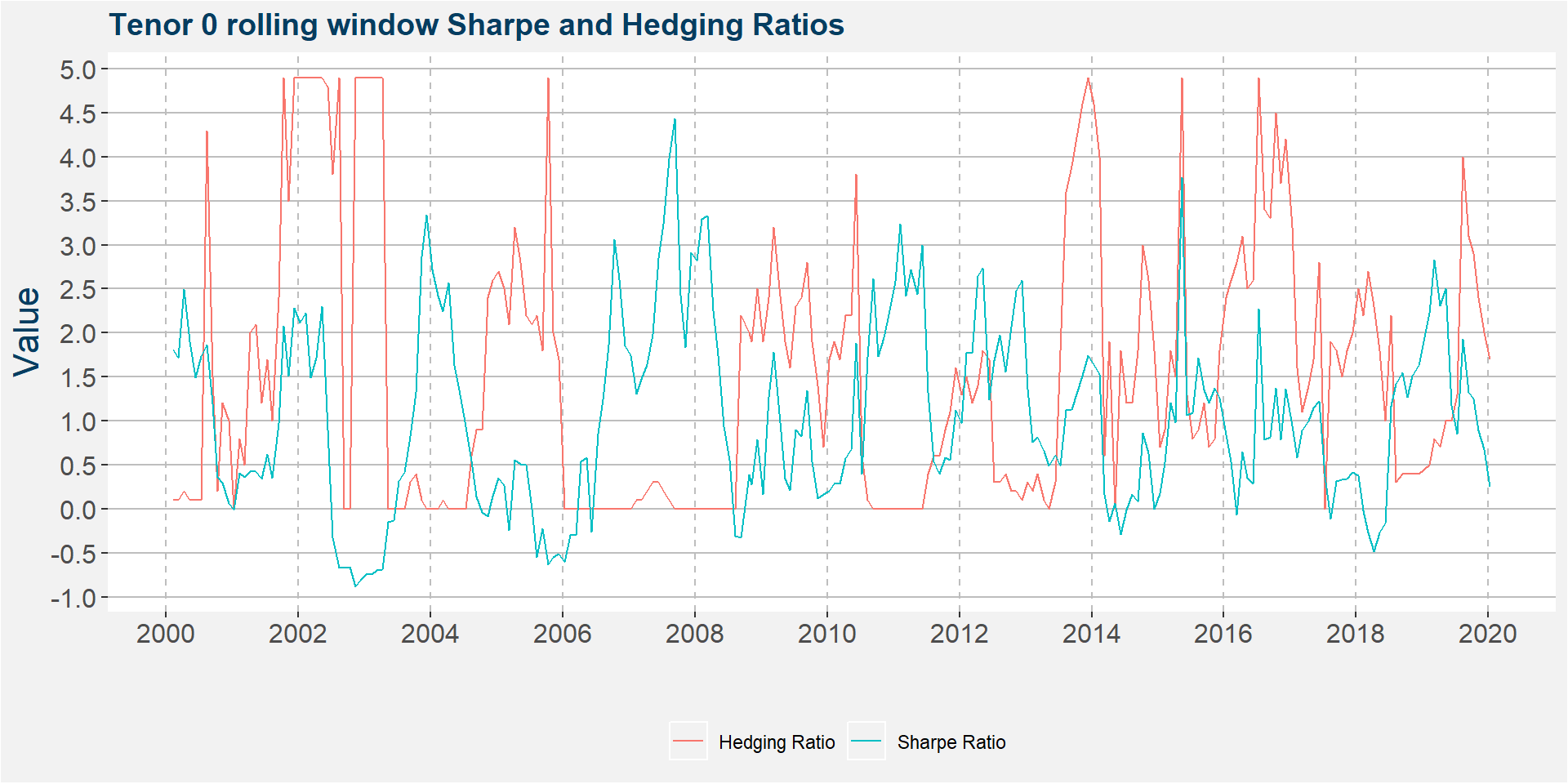
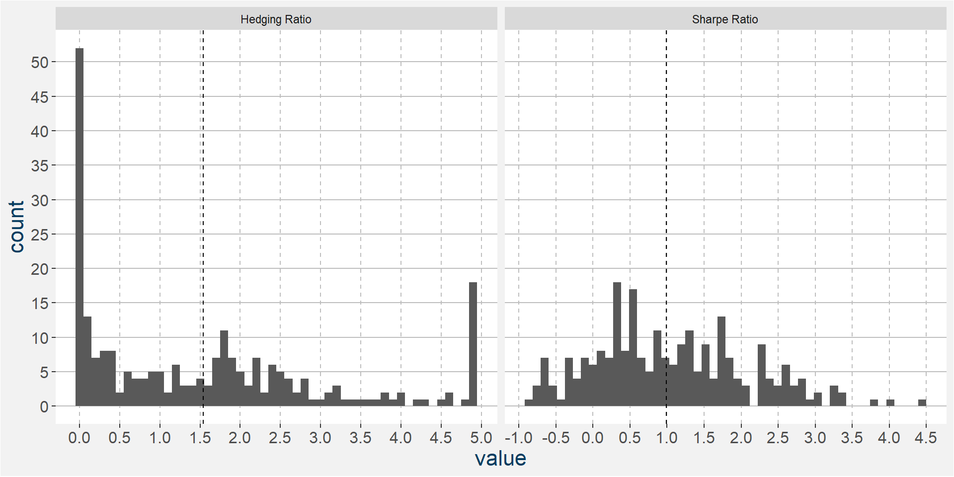
The plots below show the histograms of the hedging associated with the higherst Sharpe ratios respectively. Notice the clustering of heding ratios on the ends of the ranges. The left most cluster around \(k=0\) amounts to those cases where an outright long position in CA performed better than adding any short KW hedge. The cluster on the right hand side includes those occasions where holding a long position in CA proved to be detrimental and the hemorage can only be stopped by increasing the ratio of short KW to long CA. The dashed vertical lines represent the means of the datasets.
Cumulative Roll Adjustments
Counter to the calendar year case we see a positive slope when plotting the rolling yearly return as a function of the yearly cumulative roll adjustments. This indicated that over a larger sample the cumulative roll effect does add some value.
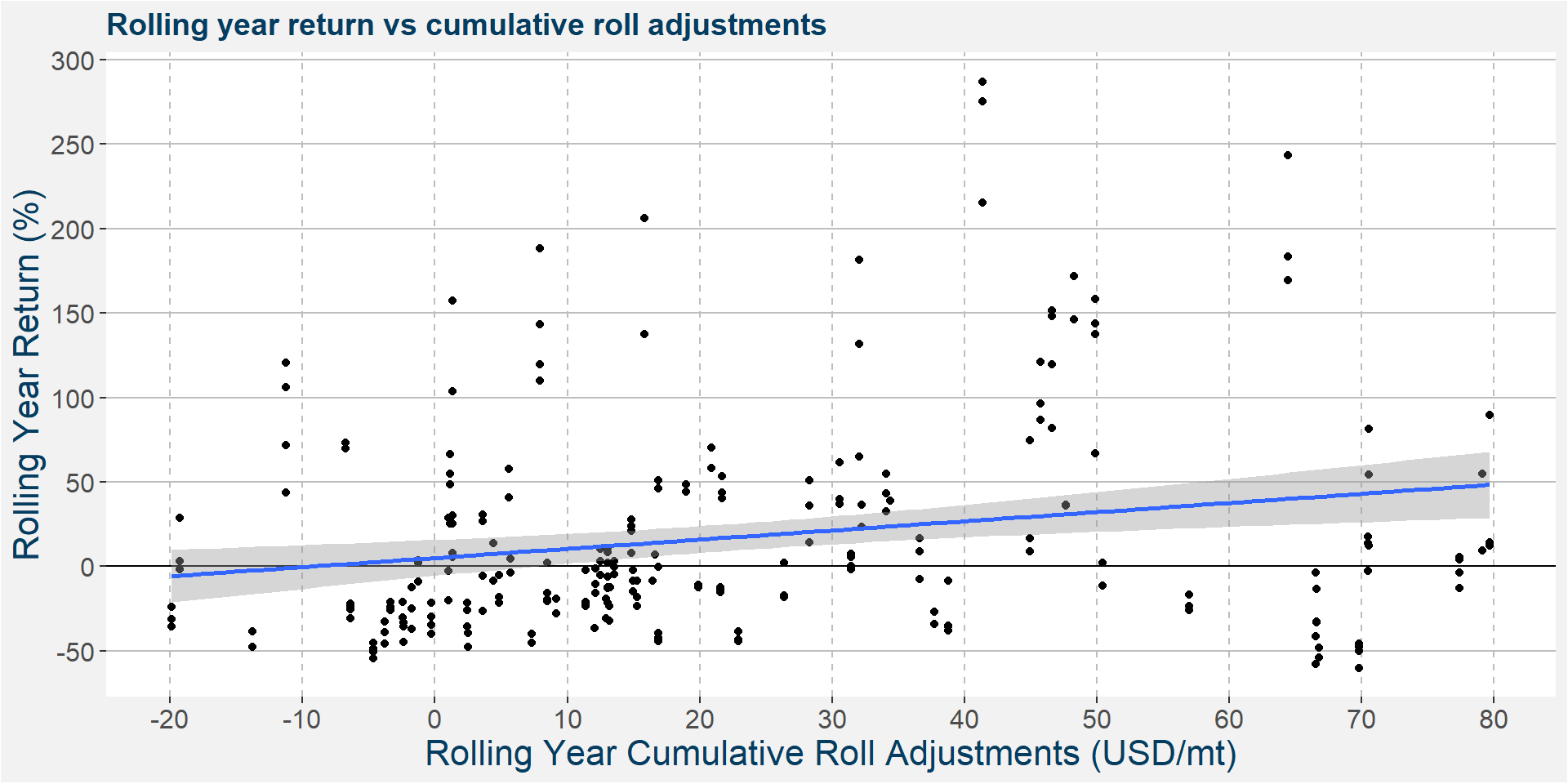
Similar to the calendar year case the table below shows the confusion matrix for the different sign of the yearly rolling returns and cumulative roll adjustments. In this case we get a whole lot more data and a better convergence of the probabilitites over a yearly rolling period.
| Return Sign | -1 | 1 | Total |
|---|---|---|---|
| -1 | 33 | 92 | 125 |
| 1 | 10 | 103 | 113 |
| Total | 43 | 195 | 238 |
Here too we can ask what is the probability of a positive yearly return given a positive roll return, which we can calculate as
\[ P( \text{Positve Yearly Return}| \text{Positive Roll Return} ) = \frac{103}{195} \approx 52.8 \%. \]
Note that the above probability is very close the the calendar year case. We can also ask what is the probability of a negative yearly return given a negative roll return, which we can calculate as
\[ P( \text{Negative Yearly Return}| \text{Negative Roll Return} ) = \frac{33}{43} \approx 76.7 \%. \]
The above finding is interesting because it shows that a negative roll has a high percentage of yielding a negative return while a positive roll gives a coin toss to a positive or negative return.
Hedging Ratio vs Cumulative Roll Adjustments
In this section we try to model the optimal hedging ratio as a functing of the cumulative roll adjustments on the rolling year basis, or at least to see if it might be possible.
The plot below shows the cumulative roll adjustments of KW and CA together with those of the spread with \(k=0.37\) as well as the \(k\)-corrected roll adjustments, these take the chosen \(k\) into account when calculating the cummulatie roll adjustments. The dashed red lines highlight the zero thresholds. For the KW and CA cumulative roll adjustments the zero line signals the break between a majority contango (less than zero) and majority backwardated (greater than zero) curve.
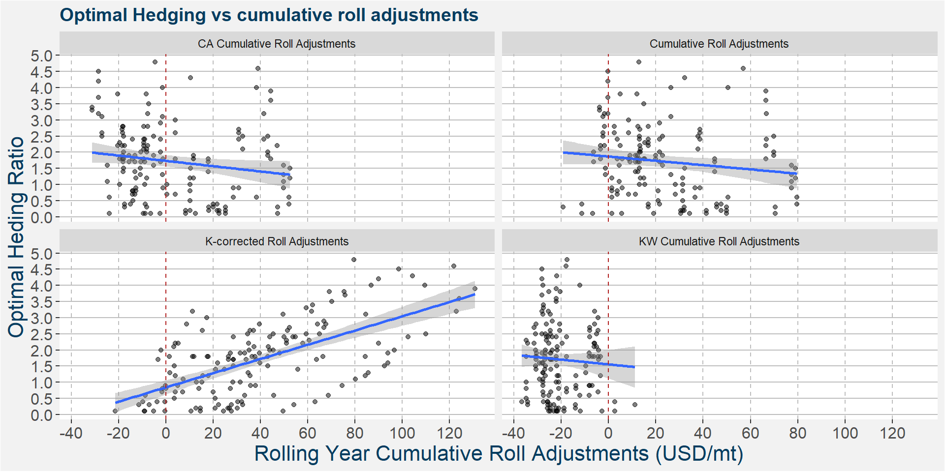
Naively we would have expected that, in the \(k=0.37\) case, the greater the cummulate roll adjustment the higher the hedging ratio shoud be. However, when we consider the top right facet we see a best fit linear curve with a negative slope, showing exactly the opposite conclusion. When correcting for the particular hedging ratios giving the optimal Sharpe ratios, bottom left facet, we see a clear upward sloping best linear fit. This implies that when a large roll return is forecasted we should consider increasing the hedging ratio.
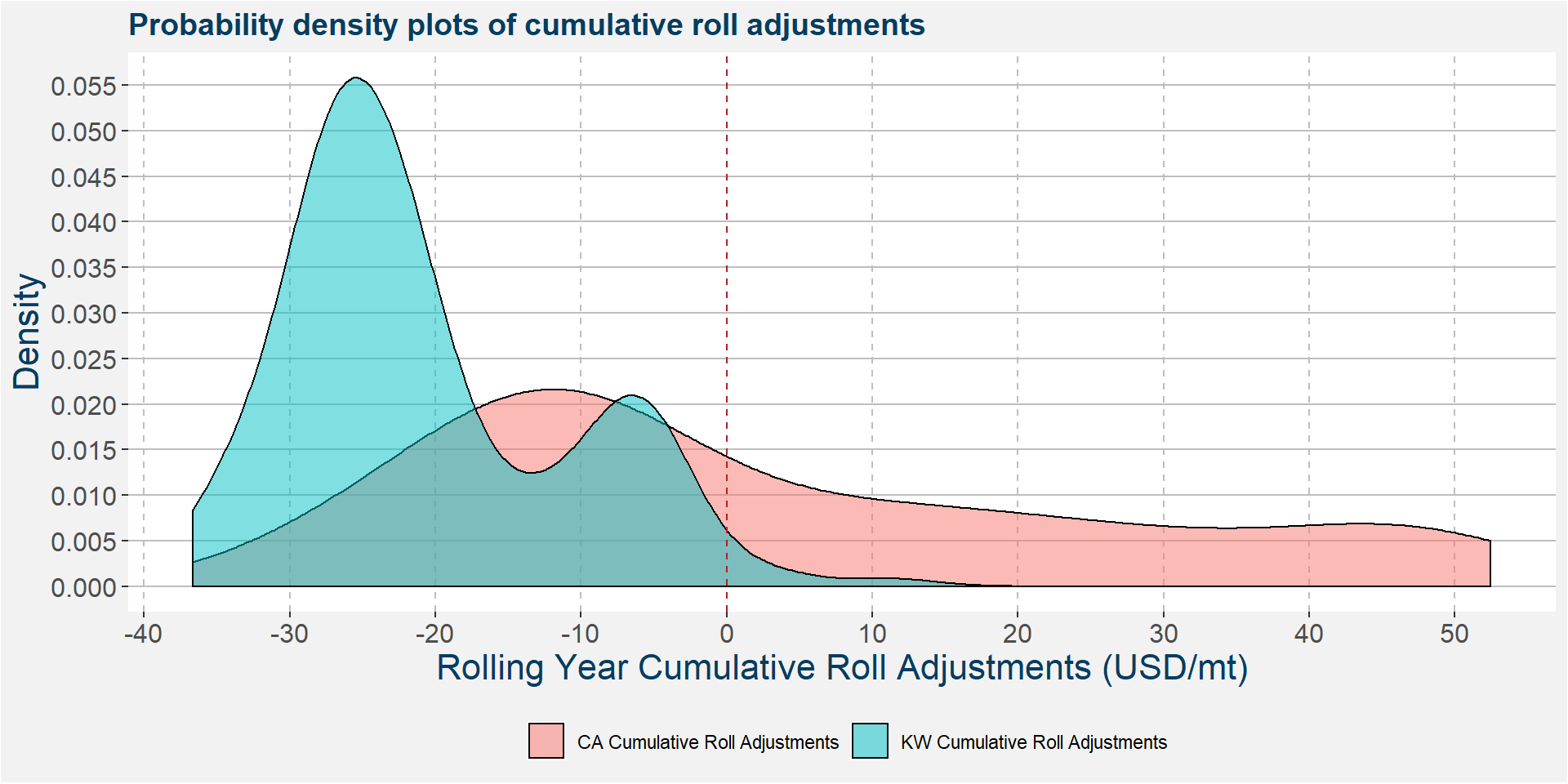
When we consider the cumulative roll adjustments of KW and CA on the same graph the differences in the roll behaviour becomes clear. From the image below we can see that KW predominantly trades in a contango and only rarely extends beyond the zero threshold. Contrast this with CA that has shown more or less a 50-50 split between contango and backwardation periods.
Consider again the top right facet plot above showing the optimal hedging ratio as a function of rolling yearly cumulative roll adjustments for the spread with \(k=0.37\). There is a gap at a cumulative roll adjustment of 60 USD/mt. To the right of the 60 USD/mt line we see those cases with large roll returns. These high roll regimes occur over prolonged periods, we split each of the contiguous regions into a separete table below. Because the KW curve was the main driver in the performance a higher hedging ratio turned out to be the best option.
The table below shows the time period from 2008-04-09 to 2009-03-11. Early on we see the CA spread being backwardated before becomming less backwardated. The KW curve remained incontango during this period and even increases the contango as time progresses. The table underneath the time frame data gives the statistics of the Sharpe and hedging ratios accross the time frame.
| Date | Sharpe | Hedging | KW Roll Adjusts | CA Roll Adjusts | Roll Adjusts | k-corrected |
|---|---|---|---|---|---|---|
| 2008-04-09 | 2.26 | 0.0 | -20.03 | 50.53 | 70.55 | 50.53 |
| 2008-05-09 | 1.74 | 0.0 | -20.03 | 50.53 | 70.55 | 50.53 |
| 2008-06-10 | 0.93 | 0.0 | -20.03 | 50.53 | 70.55 | 50.53 |
| 2008-07-11 | 0.56 | 0.0 | -19.57 | 46.98 | 66.55 | 46.98 |
| 2008-08-12 | -0.31 | 0.0 | -19.57 | 46.98 | 66.55 | 46.98 |
| 2008-09-12 | -0.32 | 2.2 | -19.57 | 46.98 | 66.55 | 90.03 |
| 2008-10-28 | 0.39 | 2.0 | -26.73 | 43.07 | 69.80 | 96.53 |
| 2008-11-10 | 0.27 | 1.9 | -26.73 | 43.07 | 69.80 | 93.86 |
| 2008-12-12 | 0.79 | 2.5 | -26.73 | 43.07 | 69.80 | 109.90 |
| 2009-01-12 | 0.17 | 1.9 | -26.73 | 43.07 | 69.80 | 93.86 |
| 2009-02-10 | 1.27 | 2.4 | -25.45 | 41.36 | 66.81 | 102.43 |
| 2009-03-11 | 1.78 | 3.2 | -25.45 | 41.36 | 66.81 | 122.79 |
| variable | Average | Stdev | p25 | Median | p75 |
|---|---|---|---|---|---|
| Sharpe | 0.7941667 | 0.8313785 | 0.245 | 0.675 | 1.3875 |
| Hedging | 1.3416667 | 1.2324833 | 0.000 | 1.900 | 2.2500 |
The table below represents the period from 2011-04-08 to 2013-08-12. Here we see strong contango periods in KW coupled with strong backwardation in CA. Notice the high hedging ratio which implies the greatest risk adjusted return was achieved with a greater short position in KW.
| Date | Sharpe | Hedging | KW Roll Adjusts | CA Roll Adjusts | Roll Adjusts | k-corrected |
|---|---|---|---|---|---|---|
| 2011-04-08 | 2.72 | 0.0 | -24.34 | 40.09 | 64.43 | 40.09 |
| 2011-05-11 | 2.44 | 0.0 | -24.34 | 40.09 | 64.43 | 40.09 |
| 2011-06-09 | 3.00 | 0.0 | -24.34 | 40.09 | 64.43 | 40.09 |
| 2011-07-12 | 1.33 | 0.4 | -27.56 | 52.13 | 79.69 | 63.15 |
| 2011-08-11 | 0.54 | 0.6 | -27.56 | 52.13 | 79.69 | 68.66 |
| 2011-09-12 | 0.40 | 0.6 | -27.56 | 52.13 | 79.69 | 68.66 |
| 2011-10-12 | 0.58 | 0.9 | -27.65 | 49.74 | 77.39 | 74.62 |
| 2011-11-09 | 0.55 | 1.1 | -27.65 | 49.74 | 77.39 | 80.15 |
| 2011-12-09 | 1.12 | 1.6 | -27.65 | 49.74 | 77.39 | 93.98 |
| 2012-01-12 | 0.97 | 1.3 | -27.65 | 49.74 | 77.39 | 85.68 |
| 2012-02-09 | 1.77 | 1.5 | -26.64 | 52.47 | 79.11 | 92.43 |
| 2012-03-09 | 1.77 | 1.2 | -26.64 | 52.47 | 79.11 | 84.43 |
| 2013-04-10 | 0.65 | 0.1 | -23.15 | 47.31 | 70.46 | 49.63 |
| 2013-05-10 | 0.49 | 0.0 | -23.15 | 47.31 | 70.46 | 47.31 |
| 2013-06-12 | 0.61 | 0.3 | -23.15 | 47.31 | 70.46 | 54.26 |
| 2013-07-11 | 0.49 | 1.8 | -22.14 | 44.47 | 66.60 | 84.31 |
| 2013-08-12 | 1.12 | 3.6 | -22.14 | 44.47 | 66.60 | 124.16 |
| variable | Average | Stdev | p25 | Median | p75 |
|---|---|---|---|---|---|
| Sharpe | 1.2088235 | 0.8426289 | 0.55 | 0.97 | 1.77 |
| Hedging | 0.8823529 | 0.9322254 | 0.10 | 0.60 | 1.30 |
What we have learned so far
- Over the entire historical sample a hedging ratio of 0.6 gives the best risk adjusted return
- The classic ton-for-ton sizing, in general, does not give the best risk adjusted return
- Much greater risk adjusted returns can be achieved during periods of positive cumulative roll
- Nagative cumulative rolls have a high (\(\approx\) 76%) probability of negative returns
- A positive cumulatie roll does not imply a positive return, which ends up beying a coin toss